4  Principles of optimization

Bayesian prior as a guide of sorts. Inspiration from Over the Garden Wall cover art. “Aint that just the way” Greg from Over the Garden Wall.

If you don’t know where you are going, you might wind up someplace else.

Yogi Berra

4.1 Optimization

General overview. Key concepts: (Get around to doing this part)

1. Local and global minimums

2. Chaotic systems

3. Gradient descent, Nelder Mead, BFGS-B, simulated annealing, cost functions.

4.2 Chaotic systems: fractals

Talk about challenges associated with dynamical systems. Initial condition sensitivity.

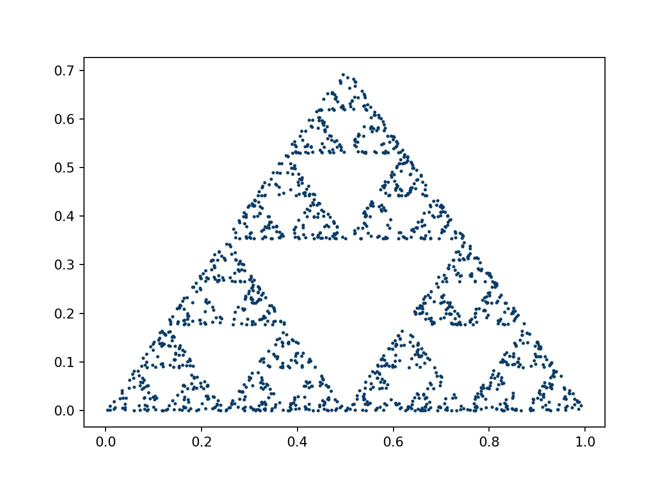
4.2.1 Sierpinski’s triangle

This code was for an assignment of Andrej Prsa’s 2018 modeling course at Villanova. Aspects of the script were borrowed from an online stackoverflow post, which is now nowhere to be found.

import numpy as np
from numpy import zeros
import warnings
warnings.filterwarnings("ignore")
import scipy.misc
import time as time
import matplotlib.pyplot as plt
import matplotlib 
from random import randint


#matplotlib.style.use('seaborn')

#sierpenski triangle
def middle(x,y,a,b):  #a and b set ratios
    return[a*(x[0]+y[0])/b,a*(x[1]+y[1])/b]
startime=time.time()
#initialize starting points
x1=[0,0]
x3=[1,0]
x2=[.5, np.sqrt(2)/2]    
current_point=[0,0]  
for i in range (1600):
    number=randint(0,2)
    if number==0:
        current_point=middle(current_point, x1,1,2)
        #current_point=[0.5*(current_point[0]+x1[0]),0.5*(current_point[1]+x1[1])]
    if number==1:
        current_point=middle(current_point, x2,1,2)
        #current_point=[0.5*(current_point[0]+x2[0]),0.5*(current_point[1]+x2[1])]
    if number==2:
        current_point=middle(current_point, x3,1,2)
        #current_point=[0.5*(current_point[0]+x3[0]),0.5*(current_point[1]+x3[1])]
    plt.scatter(current_point[0], current_point[1], s=2, c='#073d6d')
plt.show()

endtime=time.time()
print(format(endtime-startime))

15.842657327651978

4.2.2 A note on chaos vs stochasticity

Interesting distinction!

import numpy as np
import time
from numpy import zeros
import scipy.misc
import matplotlib.pyplot as plt
import matplotlib
from matplotlib import animation
import random
from random import randint
import warnings
# Comment this line out when you run it locally
warnings.filterwarnings("ignore")
plt.rcParams['animation.ffmpeg_path'] = 'ffmpeg'



starttime=time.time()
#### Vary z, keep c constant ####

#plt.imshow(mandelbrot(xpts+1j*ypts, -0.70176-0.3842j), cmap='RdBu', origin='lower')
def mandelbrot2(z, c):
    empty=np.zeros((xpts.shape[0],ypts.shape[1]))

    for i in range(225):#225 is arbitrary, but seems to get the job done, 225 times to escape
        #i believe 256 is when you get to optimal range, but this saves run time
        #especially if you have big grid
        z=z**2+c  #run num times to see if z exceeds set boundary
        empty[abs(z)<2]+=1
        #empty= abs(z) < 1  #if z is bigger than boundary, return true
    return(empty)  #run through all c values because we use grid
# set Ngrid higher for better resolution

# right now, its the number in front of j
xpts, ypts = np.ogrid[-1.5:1.5:500j, -1.9:1.9:500j]
fig,ax = plt.subplots(1)
XX=mandelbrot2(xpts+1j*ypts, -0.8+.156j)
# Make your plot, set your axes labels
ax.imshow(XX, cmap='PuBu_r', origin='lower')
ax.set_ylabel('')
ax.set_xlabel('')

# Turn off tick labels
ax.set_yticklabels([])
ax.set_xticklabels([])
#plt.imshow(mandelbrot(xpts+1j*ypts, -0.8+.156j), cmap='PuBu_r', origin='lower')
#plt.gca().axes.get_yaxis().set_visible(False)
#plt.gca().axes.get_xaxis().set_visible(False)
#change z for julia sets, change c for iconic one
#plt.xlim(-.6,.6)
#plt.ylim(-1, .25)
#plt.savefig('newmandel.pdf')
plt.show()

endtime=time.time()
print(format(endtime-starttime))

0.9011538028717041

Assignment (4.1)

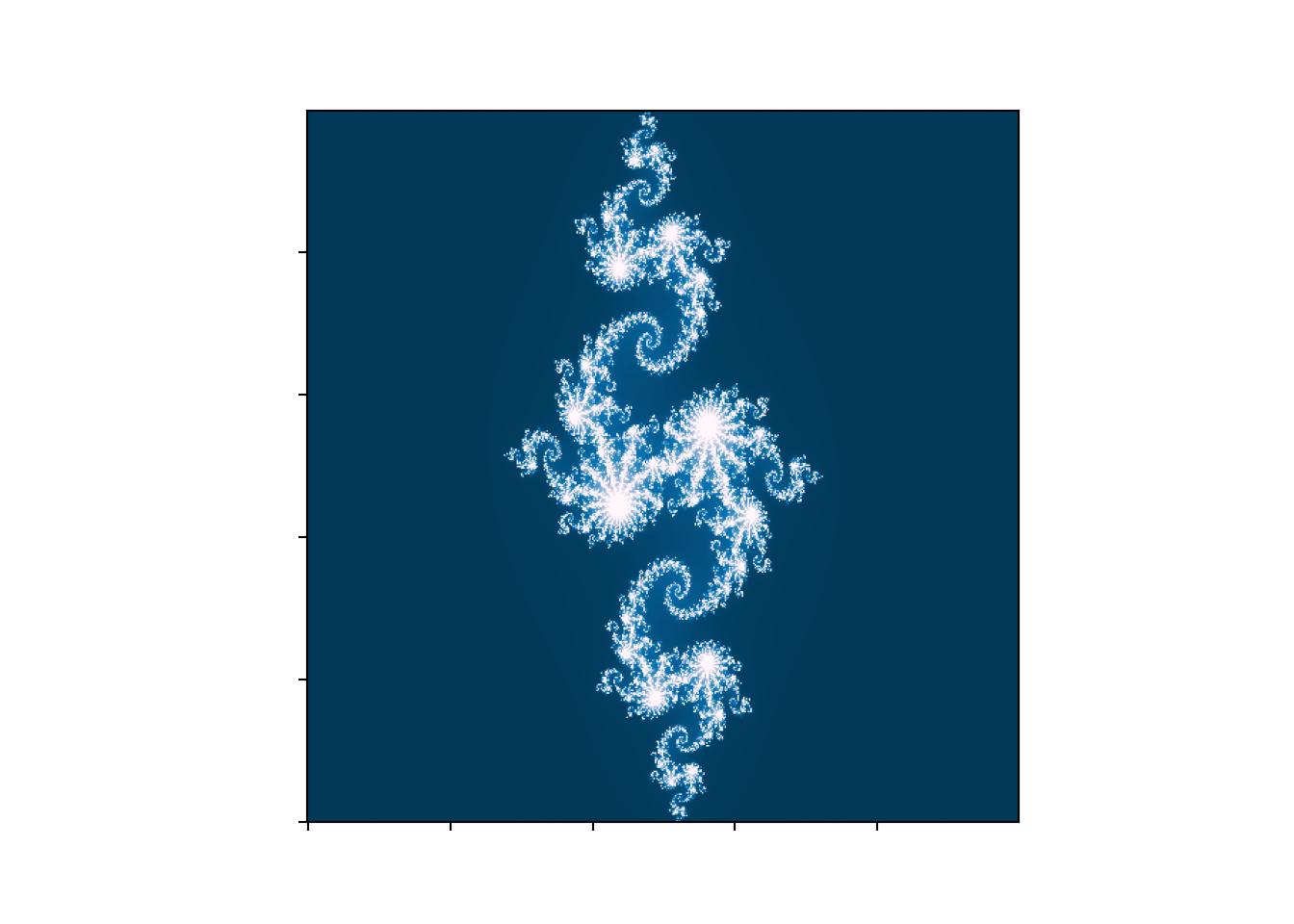
1. Instead of varying \(z\), vary \(c\) and keep \(z\) constant (this will give the more traditional Mandelbrot set image from the web). Look up different \(c\)’s that are interesting (above is called the “Julia set”).

2. Read this awesome blog/paper on the relation between fractals and neural network optimization.

3. Look up Sierpenski’s carpet and code that up.

4.2.3 The traveling salesman

The traveling salesman is a famous problem that aims to solve the following question:

“Given a list of cities and the distances between each pair of cities, what is the shortest possible route that visits each city exactly once and returns to the origin city?” wikipedia

If you have only a couple cities, a brute force approach is feasible, and, crucially, the right way to tackle the problem) However, after just a few cities, the number of combinations becomes intractable (there are \(N!\) possible combinations) and we need some sort of algorithm to search for an approximation to the best path. The approach we study here is called simulated annealing.

4.2.4 Simulated annealing

This approach is designed to find a minimum of a loss function, which here is the distance between cities. Simulated annealing is an algorithm for finding global minima/maxima. It descends from the Metropolis-Hastingsalgorithm, developed in 1953.

Informally, the algorithm follows these steps:

1. An initial path is generated, \(Q_1\), with distance \(d_1\). A random combination of the cities is also generated, \(Q_2\) with overall distance \(d_2\). This is done by swapping two distinct cities at random.

2. \(Q_1\) and \(Q_2\) are evaluated based on the distance traveled.

   a) We need to compare the new route to the old route. To do so, we generate \(u\in \text{uniform}(0,1)\) and compare \(u\) to \(e^{-(d_2-d_1)/\tau}\). If \(u<e^{-(d_2-d_1)/\tau}\), we keep the proposed swap, \(Q_2\). If not, \(Q_1\) remains the route. The temperature equation, given by \(T=T_{\text{init}}e^{-\text{temp}/\tau}\), will be updated with \(\text{temp}=\text{temp}+1\), meaning the overall temperature \(T\) will be lowered. If \(T>T_{\text{minimum}}\) , the “ending threshold”, we stop. Otherwise, repeat the procedure.

The \(T_\text{init}\) and \(T_{\text{minimum}}\) control how long the algorithm will run and can play a big role in how effective the optimization is.

What’s nice about simulated annealing is that is easily customizable. For example, if there is construction on campus, you can manually add more “cost” to that point in the algorithm by adding extra temperature at the index corresponding to that location. This has the effect of “encouraging” the algorithm to try a different route that may have a larger “actual” distance but according to our new loss function, which makes crossing the construction prohibitively expensive, is still the most efficient route, closer matching reality.

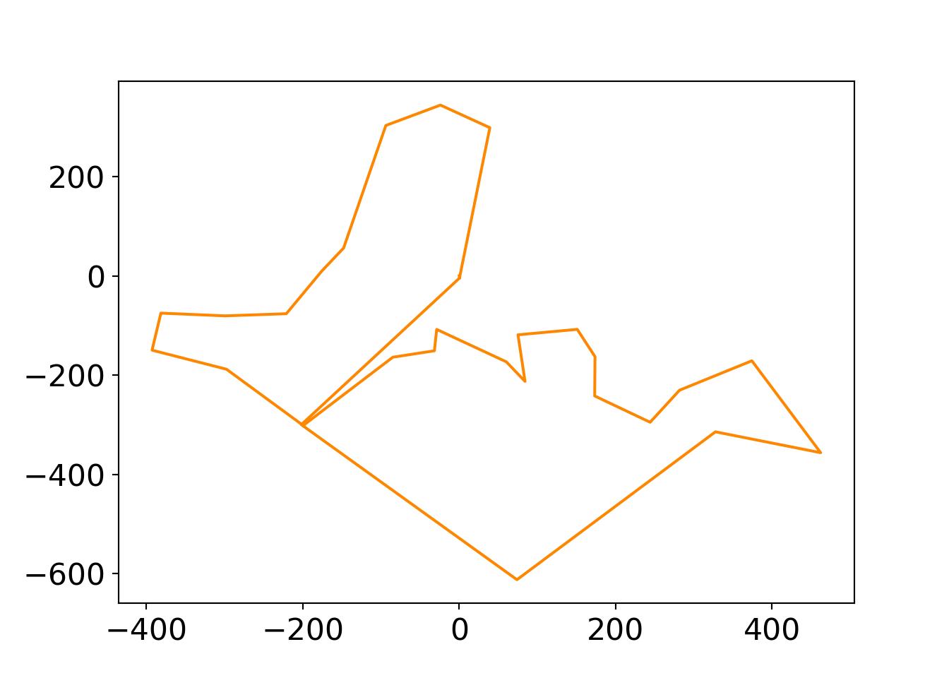
Code is adapted from the excellent “Computational Physics” by Mark Newman textbook (Newman 2013), which has a code repository This link gives a nice visual and explanation of the problem, as does this medium blog. The data are locations on Villanova University’s campus of different buildings from Jefferson Toro (in meters, with \((0,0)\) at the “geographic center” of campus).

import matplotlib
import matplotlib.pyplot as plt
from scipy.optimize import curve_fit
import numpy as np
from matplotlib import animation
from matplotlib.font_manager import FontProperties
font = {'family' : 'Fantasy',
        'weight' : 'oblique',
        'size'   : 28}
matplotlib.rc('xtick', labelsize=16) 
matplotlib.rc('ytick', labelsize=16) #changing tick size

# Set figure width to 12 and height to 9
fig_size = plt.rcParams["figure.figsize"]
fig_size[0] = 7
fig_size[1] =5
plt.rcParams["figure.figsize"] = fig_size
#matplotlib.style.use('fivethirtyeight')
import random, numpy, math
import os
os.chdir("..")
#os.getcwd()
#this time the animation will show different number of iterations
r=np.loadtxt('./quarto_bookdown/data/nova.txt')

N=len(r)-1

T_init=10  #10000 iterations
Tmin=np.array([1e-3,1e-2,1e-1,.2,.5])
tau=1e4
#magnitude of a vector
def mag(x):
    return(np.sqrt(x[0]**2+x[1]**2))
def distance():
    s=0
    for i in range(N):
        s+=mag(r[i+1]-r[i]) #distance between two cities.
    return(s)


cities1=[]  #the original points
cities2=[] # the city to visit
for i in range(N):
    cities1.append(r[i][0])
    cities2.append(r[i][1])
#r[N]=r[0]  #the last city loc is the same as first
r=np.array(r)
D=distance()



t=0
T=T_init
i=0
empty=[]
for k in range(0,5):
    while T>Tmin[k]:
        t+=1
        T=T_init*np.exp(-t/tau)
            
        i,j=random.randrange(1,N), random.randrange(1,N)
        if i==j:  #making sure the cities are distinct and swap them
            i,j=random.randrange(1,N), random.randrange(1,N)
            
        oldD=D  #previous distance
        r[i,0],r[j,0]=r[j,0],r[i,0]  #swapping the cities
        r[i,1],r[j,1]=r[j,1],r[i,1]  #swapping the cities
        D=distance()  #update distance now that positions have been updates
        deltaD=D-oldD  #want to minimize the change in distance
        u = np.random.uniform(0,1,1)
        if u>np.exp(-deltaD/T):
            r[i,0],r[j,0]=r[j,0],r[i,0]
            r[i,1],r[j,1]=r[j,1],r[i,1]
            D=oldD
        empty.append(r)
#print(D)   
#plotting and animation
newlist=[]  #the new distances
newlist2=[]

for i in range(N+1):
    newlist.append(empty[i][i][0])
    newlist2.append(empty[i][i][1])
    i+=1
newlist.append(empty[0][0][0])  #adding the final point 
newlist2.append(empty[0][1][1])  #adding the final point (return to start)
plt.plot(newlist,newlist2, color='#FD8700')



# First set up the figure, the axis, and the plot element we want to animate
fig = plt.figure()
ax = plt.axes(xlim=(-500, 500), ylim=(-700, 500))
line, = ax.plot([], [], lw=2, color='#FD8700')

# initialization function: plot the background of each frame
def init():
    line.set_data([], [])
    return line,

# animation function.  This is called sequentially
def animate(i):
    x=[]
    y=[]
    for k in range(i+1):   # we read in the first i points
        x.append(newlist[k])
        y.append(newlist2[k])
    line.set_data(x, y)
    return line,

# call the animator.  blit=True means only re-draw the parts that have changed.
anim = animation.FuncAnimation(fig, animate, init_func=init,
                               frames=N+2, interval=500)
plt.scatter(cities1,cities2, color='#012296') 



plt.text(0,10,'mendel')  
plt.text(r[2][0]+5,r[2][1]+5, 'st. marys')
plt.text(250,300, 'd=%d m'%D, fontsize=16)
plt.text(100,-600, 'south campus')
plt.xlabel('meters')
plt.ylabel('meters')

mywriter = animation.FFMpegWriter()
anim.save('./quarto_bookdown/images/travsales.mp4', writer=mywriter)
plt.close()

Assignment (4.2)

1. Find data of your campus/home/workplace/cross country road trip. Put an image of this place on the back of the plot and repeat the analysis. This blog gives a nice template for coding paths for road trips in R (Heiss 2023).

2. Mendel hall is under construction. Modify the simulated annealing code to make traversing through it prohibitively expensive, which will alter the ideal path in a hopefully sensible way.

3. BONUS: If we knew our start location and end location (a more realistic scenario), then we can use Djikstra’s algorithm. Read up on this algorithm, do a quick write-up on it, and code up (by hand or with scipy) the algorithm, starting at “Mendel Hall” and finishing at “South Campus”. This is basically building a simple GPS!

Something we want to emphasize about optimization is not to get caught up in the algorithm or the exact parameters for a specific problem you have at hand. For example, if you develop a path to travel using the simulated annealing but then find out there is a snowstorm in one of the cities, you will have to adapt your model. Not to be the harbingers of bad news, but running the simulated annealing algorithm to a higher tolerance, or trying a new algorithm will not save you in this case. The baseline model will now need to account for penalties in the snowy regions (such as a higher temperature penalty at those sites to discourage visits through those paths). However, consider the following example from Nate Silver’s “The Signal and the Noise” (Silver 2012). If everyone has a GPS that is sending them down the same path to avoid the snowstorm, then that path will now not be the most optimal¹. Now, the model will have to somehow incorporate this effect and other changes over time, such as the snowstorm moving. These are some of the difficulties facing softwares like Apple Maps or Waze. The photo below (credit to Richard Hahn for pointing this out) provides a more succinct and illuminating version of what is discussed in this paragraph.

¹ In this case, the GPS projected map becomes an “endogenous variable”, as the “model” of travel time now determines the travel time.

An interesting linkedin post on practical optimization

4.3 Optimization by hand

4.3.1 Maximum likelihood estimation

The maximum likelihood approach is a classic in frequentist statistics. It boils down the following question. Which value of the parameter makes the observed data as likely as possible? Since the parameter is considered fixed in this paradigm (and not a random variable), this approach is not an issue in any way. We will show an example where we can do this by hand (as we saw with linear regression), but typically this is done with numerical methods.

To find the MLE of the Poisson distribution,

\[\Pr(Y=y|\lambda)=\frac{e^{-\lambda}\lambda^y}{y!}\quad y=0,1,2,\ldots\]

Given \(Y_i \sim \text{Poisson}(\lambda)\) iid, what is the MLE of \(\lambda\)?

Note, the likelihood function is

\[L(\lambda|\mathbf{x})=e^{-n\lambda}\prod_{i=1}^{n}\frac{\lambda^{x_i}}{x_i}\]

Taking the log yields \[\ln L(\lambda|\mathbf{x})=-n\lambda+\sum_{i=1}^{n}x_i\ln\lambda-\sum_{i=1}^{n}\ln x_i\]

Setting the derivative with respect to \(\lambda=0\) yields

\[\begin{align*} \frac{\partial}{\partial \lambda}\ln L(\lambda|\mathbf{x})&=-n+\frac{1}{\lambda}\sum x_i\\ \hat{\lambda}&=\frac{1}{n}\sum_{i=1}^{n}x_i\\ \hat{\lambda}&=\overline{x} \end{align*} \]

Constraints can be incorporated manually through the concept of “Lagrangian multipliers”.

4.4 Decisions: utilities, risk, and loss functions

This section could very easily be its own chapters. We will try to emphasize the importance of “cost analyses”. This type of thinking is useful in the data scientists day to day, it has practical significance for choosing a model, and is even useful in the context of improving model predictive power through regularizing. For example, in “physics informed neural networks”, which we will discuss later, loss functions promote an adherence to physical constraints.

To begin, let’s just think of “loss” functions in a very informal way. If you are someone who will never fly because the worst case scenario is so horrific, you probably make decisions that optimize a different loss function than something who brings up that flying is safer than driving. So person A makes their decisions based on minimizing the worst case scenario and person B makes decisions so that on average they are safer. Person A and person B both have the same probability on the same plane of an adverse event. In fact, they both may even estimate the probability of adverse event of their potential flight as exactly the same number! Nonetheless, they chose very different actions based on their internal loss (utility) function.

Prior to formalizing these ideas, we want to mention that it is a good idea in work/life to be clear about your loss functions and how you act on them. If a company uses a minimax loss function (minimize the maximum scenario) with regard to minimizes the riskiest decisions (for example), you should know this when you get started. Many frustrations will be avoided.

Early on in the COVID-19 pandemic, the CDC was operating under a similar loss function. For example, the CDC was slow to entertain the notion that getting infected with COVID inferred some immunity. This was probably due to the fear that if the disease did not infer immunity, then guidance that previously infected people could lower their guards would be poor advice, as it would lead to further disease and strain on medical systems and general suffering. However, past experiences suggest most diseases infer some immunity, including similar diseases to COVID-19. Therefore, if public health officials were operating under an average based utility, the guidance likely would have been different. The point being is that the data and the knowledge levels may be exactly the same, but actions differ! This also helps amplify a theme of these notes: how do you define “correct”? The public official who weighed public health and social consequences to the population equally acted “correctly” if they struck a balance between total shutdowns and no public health intervention. The officials advocating for a total shutdown who was minimizing the probability of a massive amounts of death until a vaccine was available was also likely acting “correctly”². And this is due to the utility/loss function involved in decision making, a crucial point we will elaborate on further below.

² Of course, whether or not these decisions are truly optimal with respect to the utility functions is another story.

Mathematically, we can express similar ideas. A nice tool to help translate the conceptual ideas from the previous paragraph into a formal structure is through Bayes rules.

4.4.1 Bayes rules

4.4.2 Bayesian school of optimization

As we learned in the Bayesian statistics chapter, an alternative approach to searching for parameters comes through “marginalization” (loosely this means “ignoring” a certain parameter). Informally this is done by taken a weighted “sum” (weighed by the prior distribution on the parameter) of the likelihood of observed data conditioned on all the possible values of the parameter. The weighted sum is really an integral, but the big picture stays the same. The full Bayesian procedure yields a posterior probability of parameter values, “guided” by the choice of prior distribution. For a point estimate, we could take the average of the posterior draws, the mode, the median, or any statistic. As we saw before, the mean minimizes the squared error loss, and the median minimizes the absolute loss.

To implement Bayesian methods, we typically use stochastic search methods to approximate the normalizing constant integral (the “average likelihood” according to (McElreath 2018)).

4.5 Bayesian optimization

What is Bayesian optimization?

TL;DR: Bayesian optimization is a great way to optimize expensive black-box functions.

The standard ways to optimize a black-box function typically fall into one of three categories:

1. Grid search. This means trying all possible combinations of parameters for all possible values. This technique is thorough but sacrifices time. If your parameters can only take a handful of values (i.e., they are not continuous) then this may not be a bad option. This is equivalent to a for-loop.
2. Random search. Here, you define your search space and randomly sample with or without replacement a set number of times. This can be useful if the search space is large and there are limited computational resources. However, the objective function may have optima in narrow “valleys” that the random search could miss.
3. Bayesian optimization: As usual, the wikipedia page is an excellent place to start. This distill publication (Agnihotri and Batra 2020) is also a nice visualization of the basic process.

In true Bayesian fashion, the Bayesian optimization cookbook involves a prior and a posterior. The prior is over the desired function we are trying to learn, \(f(\mathbf{x})\) (see chapter 8 for a more detailed discussion of priors over functions), which after observing data, can be used to update the posterior distribution of this function, approximated by \(\hat{f}(\mathbf{x})\).

The Bayesian surrogate used for Bayesian optimization or sequential designs tends to be Gaussian processes. However, it is possible to do the same with a BART prior serving as the surrogate. To our knowledge, the first published investigation of BART for this type of work was (H. Chipman, Ranjan, and Wang 2012), who use BART for sequential design of computer experiments. In 2021, the work of (Lei et al. 2021) also use BART as a surrogate for Bayesian optimization techniques, comparing it to other leading contenders.

We will show in this vignette that the use of BART (H. A. and Chipman, George, and McCulloch 2012) for this type of study is both feasible and fairly straightforward to implement.

4.5.1 Acquisition functions

From the posterior for \(\hat{f}(\mathbf{x})\), we can define an “acquisition function”, meant to guide the search for the next point to sample. The acquisition function provides a criterion for how helpful a new input would be making the model’s output more accurate. The benefit of using a Bayesian method is we can evaluate this function over a posterior distribution of draws over the desired function \(\hat{f}(\mathbf{x})\). There are many different acquisition functions we can define, but the most common is the expected improvement.

Following the supplement of (Lei et al. 2021), we define the expected improvement as (for one dimensional \(x\) for simplicity):

\[ E\left[I(x_*)\right] = \frac{1}{M}\sum_{i=1}^{M}\left(\max\{f^m(x_*)-f^*, 0\}\right) \]

where \(f^m(x_*)\) are draws from the \(M\) BART posterior predictive distribution (where BART was trained on the input-output pair \(\{x_{1:n}, y_{1:n}\}\)), \(x_*\) are the test data, and \(f^*\) is the maximum BART prediction for the observed \(x_{1:n}\) so far (using the mean of the posterior draws for \(y_{1:n}\mid x_{1:n}\) as the point estimate). To maximize the expected improvement, we choose the \(x_*\) which leads to the highest value of the expression above for \(E\left[I(x_*)\right]\).

Hopefully this section helps emphasize the difference between Bayesianand non-Bayesian methods. Bayesian optimization is based on the concept of looking for a new input that represents the most improvement when averaged over the posterior probability of the estimated function³, which is a very Bayesian way of thinking about a problem. We search for a good next training point over a distribution of the desired function, \(f(\mathbf{x})\), evaluated at each new test point, which gives a lot of information (even if we end up taking the average improvement as our point estimate). Of course, this comes at the cost of having to specify the prior distribution, but as we argue below, using something like a BART prior mitigates that concern. This contrasts with other optimization methods which do not search over a whole distribution, but rather a single value that minimizes an objective (rewrite this paragraph).

³ which can only be defined with a specified prior

4.5.2 Benefits of a BART prior

• The implementation is fairly straightforward with the stochtree machinery, which also allows for customizability for the problem at hand (heteroskedastic forests for example).

• While choices for the priors are fairly stable off the shelf, which is generally true for BART, this requires a little more care for the sequential design realm. Due to the small sample sizes encountered in this type of study, we might need to adjust the hyper-parameters more than for other BART applications. Luckily, we probably due not need a cross-validation study or try to optimize the hyper-parameters, both of which can be costly and/or difficult to implement. In our experience, there are just a few knobs we can adjust that allow us to converge upon a decent fit pretty quickly. We share some suggestions in the table below: (Delete this probably)

  Hyper-parameter	Change from default	Intended effect	Use case
  Tree growing process: \(\alpha\), \(\beta\)	alpha smaller, beta larger	Smaller trees	Lower signal/higher noise data. Stronger regularization to avoid overfitting.
  	alpha bigger, beta smaller	Bigger trees	Less regularized, useful if we expect higher order interactions but can overfit easier.
  \(\sigma^2\) parameter (from \(\varepsilon\sim N(0,\sigma^2)\)	a_leaf larger, b_leaf smaller (or set sigma2_init closer to 0)	Smaller error standard deviation	Similar to less regularization on trees, useful alternative to changing those priors when dealing with small sample sizes, can lead to overfitting
  	a_leaf smaller, b_leaf larger (or set sigma2_init higher)	Larger error standard deviation	Conservative, can underfit
  Variable split location granularity	cutpoint_grid_size		Maybe if you have a variable with a very wide range
  Leaf node parameters	k higher	smoother estimates	More shrinkage/regularization.
  	min_samples_leaf lower	more splits potentially	useful with small sample sizes to avoid not being to make splits, can overfit
  Number of trees	num_trees higher	smoother estimates	Useful if we expect smoothness, or more complicated signal that is difficult to decipher. Too high can lead to over-fitting
  	num_trees lower	remove redundant trees	Useful as a baseline surrogate for “fitting the fit procedures” (Carvalho et al. 2021), or if the pattern is expected a priori simpler to learn.

4.5.3 1-D Simulated example

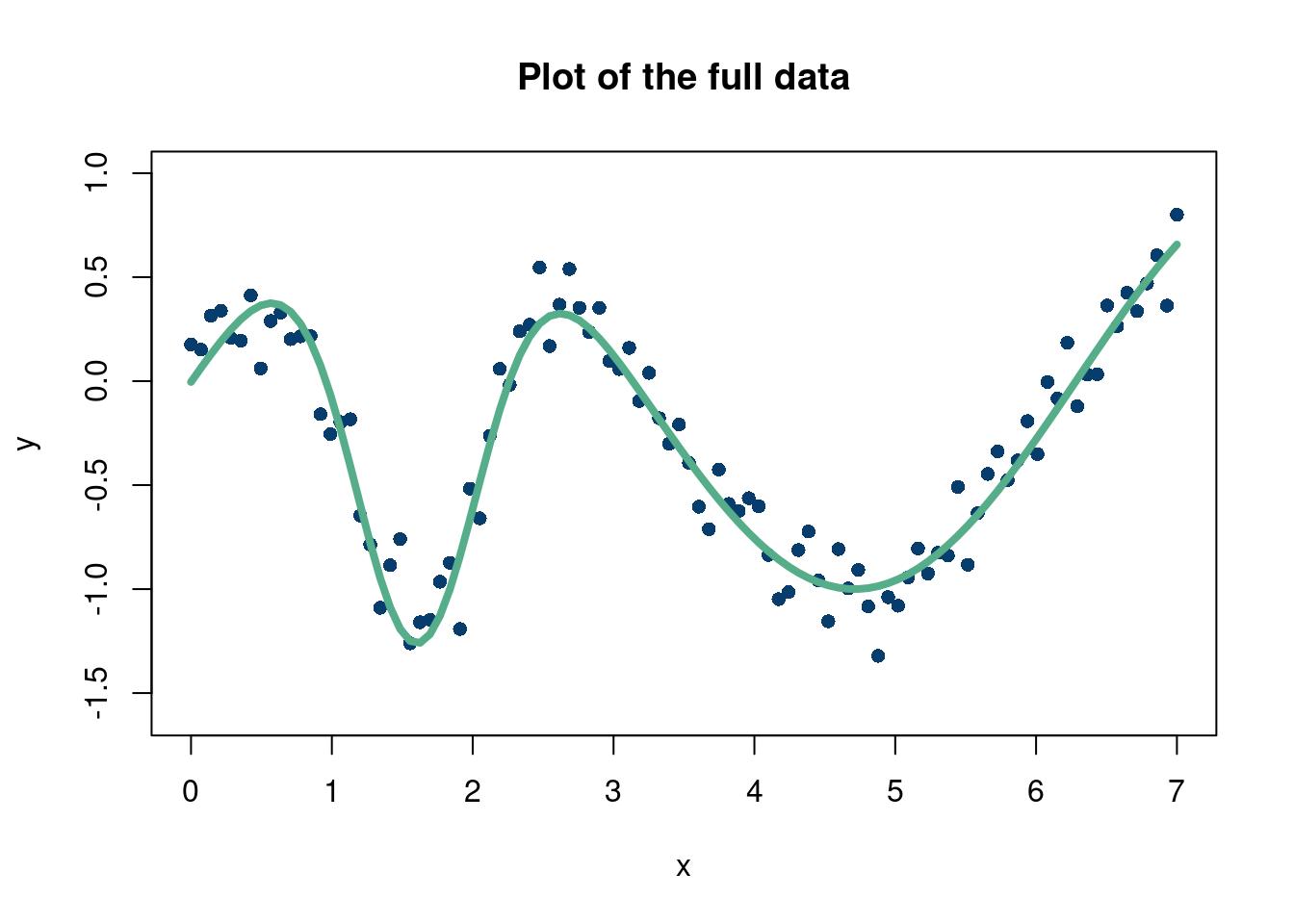
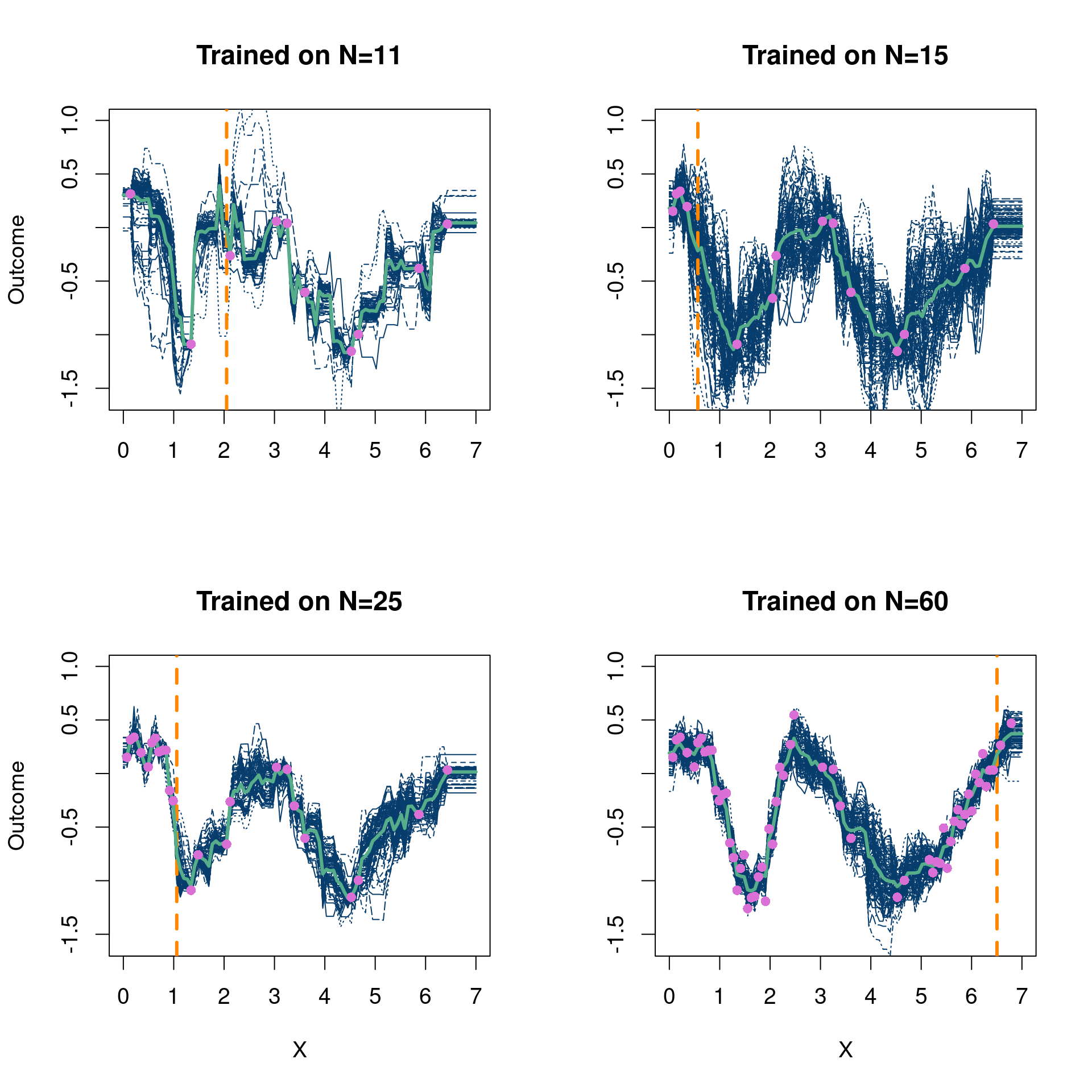
This example is from chapter 7 of Surrogates (Gramacy 2020). We perform the BO algorithm starting with 10 input points and select the “Most improved” points from a grid of 100 points that we test the trained BART output on (meaning we train on 10 points initially and jump to the next \(x\) value which will improve the prediction the most on average).

options(warn=-1)
suppressMessages(library(stochtree))
suppressMessages(library(gganimate))
suppressMessages(library(tidyverse))
suppressMessages(library(dplyr))

num_gfr <- 20
num_burnin <- 10
num_mcmc <- 100
num_samples <- num_gfr + num_burnin + num_mcmc


RMSE <- function(m, o){
  sqrt(mean((m - o)^2))
}
# start with 10 points randomly selected
design_init = 10
N = 100
set.seed(12024)
RMSE_list = matrix(NA, nrow=50, ncol = 1)


 fsindn <- function(x)
 sin(x) - 2.55*dnorm(x,1.6,0.45)
# consistent X
 X = matrix(seq(from=0, to=7, length.out=N))
 X_full = X
 y <- fsindn(X) + rnorm(length(X), sd=0.15)
 first_guess = sample.int(nrow(X), design_init)
 # The data
 plot(X, y, xlab="x", ylab="y", ylim=c(-1.6,1),col='#073d6d', pch=16, cex=1, main='Plot of the full data')
  lines(X, fsindn(X), xlab="x", ylab="f(x)", ylim=c(-1.6,1),col='#55AD89',lwd=4, pch=16, cex=0.75, main='True function without noise')

 # For plotting purposes
BART_fit = c()
next_step = c()
X_train_sub = c()
y_train_sub = c()
for (k in 1:50){
# remove these X's
new_X = setdiff(seq(from=1, to=nrow(X)), first_guess)
# your initial X's
X_train = as.matrix(X[first_guess,])
X_test = X_full#as.matrix(X[new_X,])
y_train = y[first_guess]
y_test = y#[new_X]



bart_model_warmstart <- stochtree::bart(
    X_train = X_train, y_train = y_train, X_test = X_test, 
     num_gfr = num_gfr, num_burnin = num_burnin, #alpha=0.995, beta=1.25,
    num_mcmc = num_mcmc, 
    mean_forest_params = list(
      num_trees = 100,
    min_samples_leaf=1, sigma2_init=1e-2,
 sigma2_leaf_shape = 6, sigma2_leaf_scale = 0.25
))
# the maximum of f up until now
f_max = max(rowMeans(bart_model_warmstart$y_hat_train))
EI = sapply(1:length(new_X), function(j) (1/num_mcmc)*sum(sapply(1:num_mcmc, function(i)max((bart_model_warmstart$y_hat_test[j,i]-f_max),0))))

most_improved = new_X[which(EI==max(EI))]
if(length(most_improved) > 1){
  most_improved <- sample(most_improved, 1)
}
first_guess = c(first_guess, most_improved)
RMSE_list[k, 1] = RMSE(rowMeans(bart_model_warmstart$y_hat_test), y_test)
BART_fit[[k]] = (bart_model_warmstart$y_hat_test)
next_step[[k]] = X_test[most_improved,]
X_train_sub[[k]] = X_train
y_train_sub[[k]] = y_train
}
 BART_means = unlist(lapply(1:50, function(i)rowMeans(BART_fit[[i]])))
 train_size = unlist(lapply(11:60, function(k)rep(k, length(X_test)*num_mcmc)))
 X_seq = rep(rep(X_test, num_mcmc), 50)
 mcmc_draw = unlist(lapply(1:num_mcmc, function(q)rep(q, length(X_test))))
mcmc_draw = rep(mcmc_draw, 50)
BART_fits = unlist(lapply(1:50, function(q)c(unlist(BART_fit[[q]]))))
 df_plot = data.frame(X = X_seq,BART_fit = BART_fits,  iteration=train_size , mcmc_draw=mcmc_draw)
 
# https://stackoverflow.com/questions/77532571/use-dropdown-menu-to-print-different-ggplotly-plots-in-rmarkdown
ani_BO = ggplot(df_plot,aes(x=X, y=BART_fit, group=mcmc_draw))+

      transition_time(
    as.integer(iteration)
  ) +
    geom_line(col='#073d6d', lwd=0.04, alpha=0.7)+stat_summary(aes(x=X, y=BART_fit, group=F),fun = "mean", colour = "#55AD89", size = 1.75, geom = "line")+xlab('X')+ylab('predicted outcome')+
    labs(title = 'Training size: {frame_time}')+ theme_minimal()+ theme(plot.title = element_text(hjust = 0.5), 
        text = element_text(size = 16))

#ani_BO <- animate(ani_BO, renderer = ffmpeg_renderer(),
#                  width = 630, height = 450,nframes = 50, fps=4)
#anim_save(paste0(here::here(),'/images/BART_BO.mp4'), ani_BO)

An animation of the BART Bayesian optimization procedure.

For a cleaner visual, we can do this in base R as well. The the orange dashed line in the plot below is the “next point” sampled.

 par(mfrow=c(2,2), cex=1.22)
  matplot(X_test,BART_fit[[1]], pch=16, col='#073d6d', type='l', lwd=1.0, ylim=c(-1.6,1),xlab='', ylab='Outcome',main=paste0('Trained on N=', design_init+(1)))
abline(v=c(next_step[[1]]), lty=2, lwd=3, col='#FD8700')
lines(X_test,rowMeans(BART_fit[[1]]), col='#55AD89', lwd=3, lty=1)
points(X_train_sub[[1]],y_train_sub[[1]], col='#Da70D6', type='p', cex=0.95, pch=16)
#legend('topright', c('Posterior draws', 'Mean BART fit', 'training data'), pch = c(16,16), lty=c(1,1), lwd=3, col=c('#073d6d','#Da70D6', '#55AD89', '#FD8700'),
#       bg='white')


  matplot(X_test,BART_fit[[5]], pch=16, col='#073d6d', type='l', lwd=1.0, ylim=c(-1.6,1),main=paste0('Trained on N=', design_init+(5)),
          xlab='', ylab='')
abline(v=c(next_step[[5]]), lty=2, lwd=3, col='#FD8700')
lines(X_test,rowMeans(BART_fit[[5]]), col='#55AD89', lwd=3)

points(X_train_sub[[5]],y_train_sub[[5]], col='#Da70D6', type='p', cex=0.95, pch=16)

  matplot(X_test,BART_fit[[15]],ylim=c(-1.6,1), pch=16, col='#073d6d', type='l', lwd=1.0, main=paste0('Trained on N=', design_init+(15)), 
          xlab='X', ylab='Outcome')
abline(v=c(next_step[[15]]), lty=2, lwd=3, col='#FD8700')
lines(X_test,rowMeans(BART_fit[[15]]), col='#55AD89', lwd=3)
points(X_train_sub[[15]],y_train_sub[[15]], col='#Da70D6', type='p', cex=0.95, pch=16)


  matplot(X_test,BART_fit[[50]], ylim=c(-1.6,1), pch=16, col='#073d6d', type='l', lwd=1.0, main=paste0('Trained on N=', design_init+(50)), 
          xlab='X', ylab='',)
abline(v=c(next_step[[50]]), lty=2, lwd=3, col='#FD8700')
lines(X_test,rowMeans(BART_fit[[50]]), col='#55AD89', lwd=3)

points(X_train_sub[[50]],y_train_sub[[50]], col='#Da70D6', type='p', cex=0.95, pch=16)

Figure 4.1: Notice, we see some bunching…

So we start off fitting this (admittedly easy) function pretty well with only 10 data points, but pretty quickly converge to the real function. Excellent. The dashed orange line in Figure 4.1 shows the next location that is added to the training data for the next BART fit.

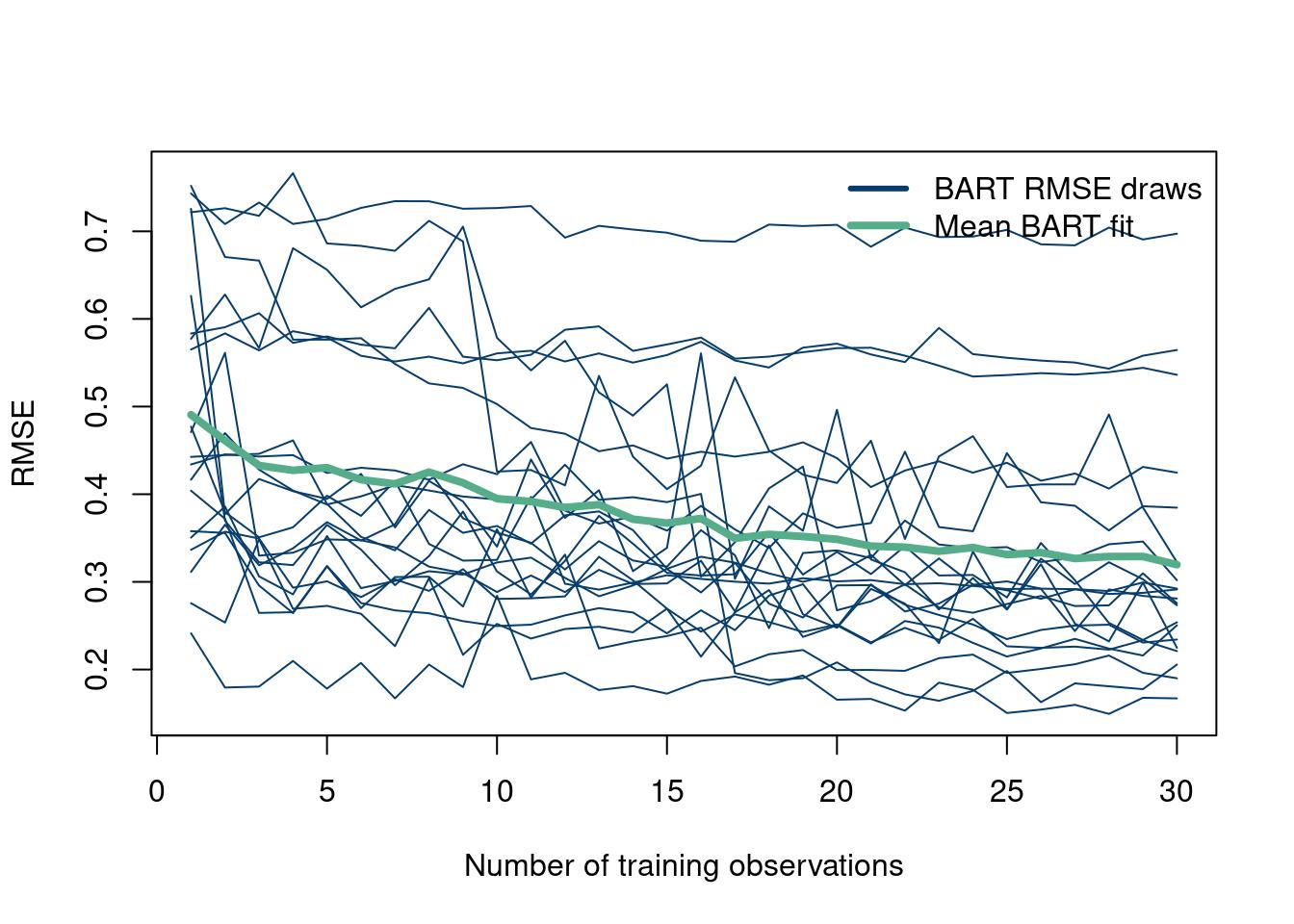
4.5.4 Monte Carlo repetitions

Now, we repeat the experiment 20 times just to make sure this particular set of Monte Carlo draws were not just an easy realization of the DGP. This is fairly easy, as it just requires wrapping the inner loop with one outer loop. Just so it does not take too long, we only do 20 repetitions (with only 10-40 training points to save compute time), but crank this number up.

suppressMessages(library(stochtree))

num_gfr <- 10
num_burnin <- 100
num_mcmc <- 50
num_samples <- num_gfr + num_burnin + num_mcmc


RMSE <- function(m, o){
  sqrt(mean((m - o)^2))
}
# start with 10 points randomly selected
design_init = 10
N = 100
num_rep = 20
RMSE_list = matrix(NA, nrow=30, ncol = num_rep)
GP_RMSE = matrix(NA, nrow=N-design_init, ncol = num_rep)
for (M in 1:num_rep){
 fsindn <- function(x)
 sin(x) - 2.55*dnorm(x,1.6,0.45)
# consistent X
 X = matrix(seq(from=0, to=7, length.out=N))
 X_full = X
 y <- fsindn(X) + rnorm(length(X), sd=0.15)
 first_guess = sample.int(nrow(X), design_init)


 # For plotting purposes
BART_fit = c()
next_step = c()
X_train_sub = c()
y_train_sub = c()
for (k in 1:30){
# remove these X's
new_X = setdiff(seq(from=1, to=nrow(X)), first_guess)
# your initial X's
X_train = as.matrix(X[first_guess,])
X_test = X_full#as.matrix(X[new_X,])
y_train = y[first_guess]
y_test = y#[new_X]



bart_model_warmstart <- stochtree::bart(
    X_train = X_train, y_train = y_train, X_test = X_test, 
    num_gfr = num_gfr, num_burnin = num_burnin, #alpha=0.995, beta=1.25,
    num_mcmc = num_mcmc, 
    general_params = list(sigma2_global_init = 1e-2, sigma2_global_scale = 1e-3),
    mean_forest_params = list(
      num_trees = 100,
    min_samples_leaf=1, sigma2_leaf_init=1e-1,
 sigma2_leaf_shape = 6, sigma2_leaf_scale = 0.25
)
)
# the maximum of f up until now
f_max = max(rowMeans(bart_model_warmstart$y_hat_train))
EI = sapply(1:length(new_X), function(j) (1/num_mcmc)*sum(sapply(1:num_mcmc, function(i)max((bart_model_warmstart$y_hat_test[j,i]+bart_model_warmstart$sigma2_global_samples[i]*rnorm(1)-f_max),0))))

most_improved = new_X[which(EI==max(EI))]
if(length(most_improved) > 1){
  most_improved <- sample(most_improved, 1)
}
first_guess = c(first_guess, most_improved)
RMSE_list[k, M] = RMSE(rowMeans(bart_model_warmstart$y_hat_test), y_test)


}
}
matplot(RMSE_list, type='l', col='#073d6d', lwd=1, ylab='RMSE', xlab='Number of training observations', lty=1)

matpoints(rowMeans(RMSE_list), type='l', lwd=4, col='#55AD89')

legend("topright", c("BART RMSE draws", "Mean BART fit"), col=c('#073d6d', '#55AD89'), lty=c(1,1),bty="n", lwd=c(3,4))

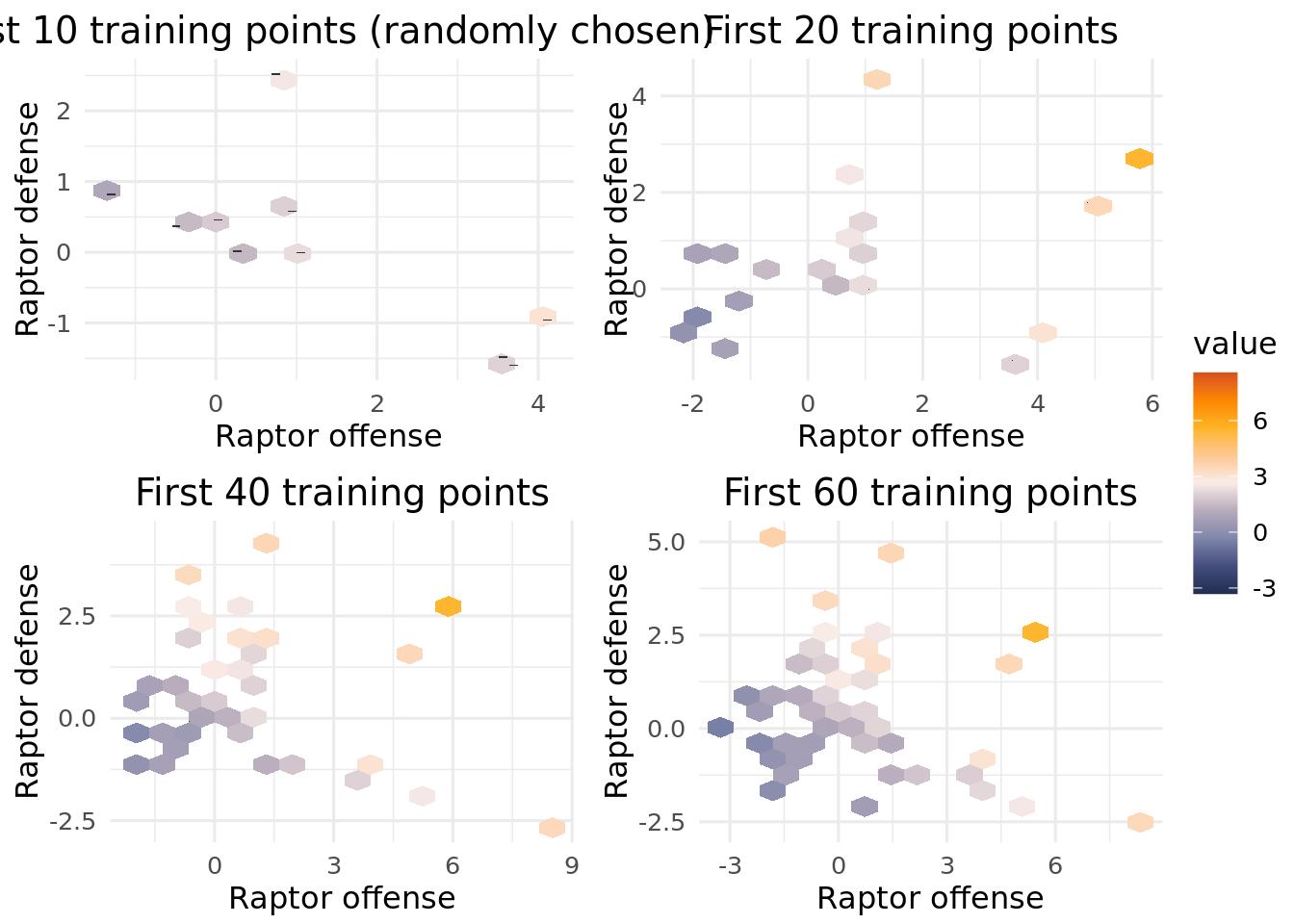
4.5.5 A 2-D example on real data

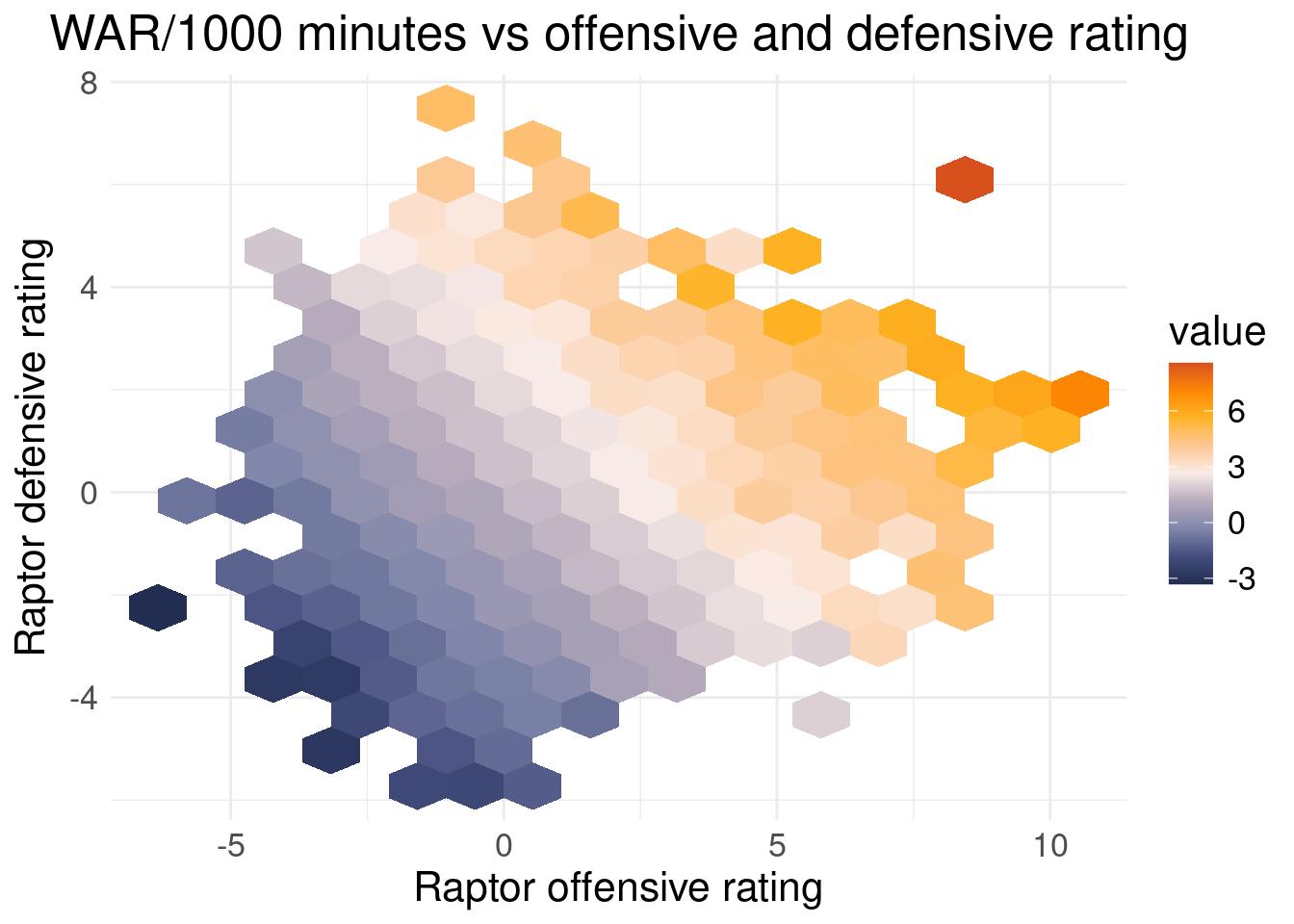
You are curious in FiveThirtyEights RAPTOR projections, particularly in how WAR is calculated (a metric for wins above replacement, mean to quantify a player’s value). The data include a player’s offensive rating, their defensive rating, minutes played, and their overall value. Unbeknownst to you, the data are published in csv format on the fivethirtyeight github repo. You think you can only find the data on the interactive published webpage, and think you need to manually load the data into a local CSV one by one, a tedious task.

Here comes Bayesian optimization! After recording a few observations, you feed the data to the Bayesian optimization algorithm, and try and learn the relationship between offensive and defensive rating as inputs, and WAR/thousand minutes as output⁴. We filter out players with less than 1000 minutes, which means we are excluding players who missed significant time or players who were not major contributors (~15 minutes per game for an 82 game season). We do not sample the error term, \(\sigma^2\), and set its initial value close to \(0\). Theoretically, WAR is calculated deterministically, so the uncertainty should arise from limited data, not measurement error.

⁴ To account for different playing times, you divide by minutes played to get WAR/minutes to level the playing field. Multiply by 1000 because that’s our minimum minute threshold.

options(warn=-1)
suppressMessages(library(dplyr))
suppressMessages(library(tidyverse)) 
suppressMessages(library(GGally))
suppressMessages(library(plotly))
suppressMessages(library(NatParksPalettes))
suppressMessages(library(gganimate))
suppressMessages(library(stochtree))


RMSE <- function(m, o){
  sqrt(mean((m - o)^2))
}
nba_ratings = read.csv(paste0(here::here(), "/data/modern_RAPTOR_by_player.csv"))
#nba_ratings = read.csv('https://raw.githubusercontent.com/fivethirtyeight/data/refs/heads/master/nba-raptor/modern_RAPTOR_by_player.csv')
# Filter out players with less than 1000 minutes played in a season.
nba_ratings  = nba_ratings %>%
  dplyr::filter(mp>1000)


num_gfr <- 10
num_burnin <- 10
num_mcmc <- 100
num_samples <- num_gfr + num_burnin + num_mcmc
X = as.matrix(nba_ratings[,c('raptor_box_offense', 
          'raptor_box_defense')])
test_set_pct <- 0.2
n_test <- round(test_set_pct*nrow(X))
n_train <- nrow(X) - n_test
test_inds <- sort(sample(1:nrow(X), n_test, replace = FALSE))
train_inds <- (1:nrow(X))[!((1:nrow(X)) %in% test_inds)]
X_train = X[train_inds,]
X_test = X[test_inds,]
y_train = 1000*nba_ratings$war_reg_season[train_inds]/nba_ratings$mp[train_inds]
y_test = 1000*nba_ratings$war_reg_season[test_inds]/nba_ratings$mp[test_inds]
bartFit <- stochtree::bart(X_train= X_train,
                           y_train = y_train,
                           X_test = X_test,
                           num_gfr = num_gfr, num_burnin = num_burnin, #alpha=0.995, beta=1.25,
                           num_mcmc = num_mcmc, 
                           general_params = list(sample_sigma2_global=F, 
                                                 sigma2_global_init=1e-3),
                            mean_forest_params = list(
      num_trees = 200,
    min_samples_leaf=1, sigma2_init=1e-1,
 sigma2_leaf_shape = 6, sigma2_leaf_scale = 0.5
))
plot(rowMeans(bartFit$y_hat_test), y_test, pch=16, col='#1d2951' )
abline(a=0, b=1, col='#E3120B')

# Baseline
print(paste0('The RMSE for the full data is: ',round(RMSE(rowMeans(bartFit$y_hat_test), y_test),2)))

[1] "The RMSE for the full data is: 0.58"

# to store results
num_rep = 20
# start with 15 points randomly selected
design_init = 10
N = 60
set.seed(12024)
RMSE_list = matrix(NA, nrow=N-(design_init-1), ncol = 1)


# consistent X
X_full = X
y = 1000*(nba_ratings$war_reg_season/nba_ratings$mp)

first_guess = sample.int(nrow(X), design_init)

print(paste0(nba_ratings[first_guess, c('player_name')], '_',
       nba_ratings[first_guess, c('season')]))

 [1] "Chris Duarte_2022"    "Isaiah Thomas_2016"   "Al-Farouq Aminu_2014"
 [4] "Al Horford_2020"      "Greg Monroe_2015"     "Courtney Lee_2014"   
 [7] "Tre Jones_2022"       "Miles Bridges_2022"   "Damian Lillard_2014" 
[10] "James Harden_2022"   

# For plotting purposes
BART_fit = c()
next_step = c()
X_train_sub = c()
y_train_sub = c()

for (k in 1:(N-design_init)){
  # remove these X's
  new_X = setdiff(seq(from=1, to=nrow(X)), first_guess)
  # your initial X's
  X_train = as.matrix(X[first_guess,])
  X_test = X_full#as.matrix(X[new_X,])
  y_train = y[first_guess]
  y_test = y#[new_X]
  
  
  
  bart_model_warmstart <- stochtree::bart(
    X_train = X_train, y_train = y_train, X_test = X_test, 
     num_gfr = num_gfr, num_burnin = num_burnin, #alpha=0.995, beta=1.25,
        num_mcmc = num_mcmc,
    mean_forest_params = list(min_samples_leaf=1, sigma2_init=5e-2,
 sigma2_leaf_shape=6, sigma2_leaf_scale=0.5,num_trees = 200)
  )
  # the maximum of f up until now
  f_max = max(rowMeans(bart_model_warmstart$y_hat_train))
  EI = sapply(1:length(new_X), function(j) (1/num_mcmc)*sum(sapply(1:num_mcmc, function(i)
    max((bart_model_warmstart$y_hat_test[j,i]-f_max),0))))
  
  most_improved = new_X[which(EI==max(EI))]
  if(length(most_improved) > 1){
  most_improved <- sample(most_improved, 1)
}
  first_guess = c(first_guess, most_improved[1])
  RMSE_list[k, 1] = RMSE(rowMeans(bart_model_warmstart$y_hat_test), y_test)
  BART_fit[[k]] = (bart_model_warmstart$y_hat_test)
  next_step[[k]] = X_test[most_improved,]
  X_train_sub[[k]] = X_train
  y_train_sub[[k]] = y_train
}


#train_size = seq(from=1,to=100, by=5)
train_size = seq(from=1, to=(N-design_init))
preds = unlist(lapply(train_size, 
                      function(i)rowMeans(BART_fit[[i]])))
iteration = unlist(lapply(train_size+10, function(i)
  rep(i, nrow(X))))
df2 = data.frame(pred = preds, box_off=rep(X[,1],length(train_size)), 
                 box_def=rep(X[,2],length(train_size)), iteration=iteration)

a2 = ggplot(df2, aes(box_off, box_def, z= pred)) + 
  transition_time(
    as.integer(iteration)
  ) +
  stat_summary_hex(fun = function(x) quantile(x, 0.50), 
                   bins = 16) +
  
  #geom_point(size=3.25)+
  scale_fill_gradientn(colors=NatParksPalettes::natparks.pals("Acadia"), # Instead, could use MetBrewer::met.brewer('Kandinsky')
            limits=c(min(y), 
                     max(y)))+
  labs(title = 'Training size: {frame_time}')+ 
  xlab('Raptor offensive rating')+ylab('Raptor defensive rating')+
  #ggtitle(paste0('Training size = ',design_init))+
  theme_minimal()+
  theme(plot.title = element_text(hjust = 0.5), 
        text = element_text(size = 16))

#a3 <- animate(a2, renderer = ffmpeg_renderer(), width = 700, height = 500)#, options(gganimate.dev_args = list(bg = 'transparent')))
#anim_save(paste0(here::here(),'/images/NBA_BO_anim.mp4'), a3)

Looking at the full relationship vs the Bayesian optimized fit with more training data:

df4 = ggplot(nba_ratings, aes(raptor_box_offense, raptor_box_defense,
                        z = 1000*(war_reg_season/mp))) +
  stat_summary_hex(fun = function(x) quantile(x, 0.50), 
                   bins = 16) +
  
  #geom_point(size=1)+
  geom_tile()+scale_fill_gradientn(colors=natparks.pals("Acadia"))+
  ggtitle('WAR/1000 minutes vs offensive and defensive rating')+  xlab('Raptor offensive rating')+ylab('Raptor defensive rating')+
  theme_minimal()+
  theme(plot.title = element_text(hjust = 0.5), 
        text = element_text(size = 16))
df4

#ggsave(paste0(here::here(), '/images/BO_2D_truth.svg'), df4, height=5, width=7, bg='transparent')

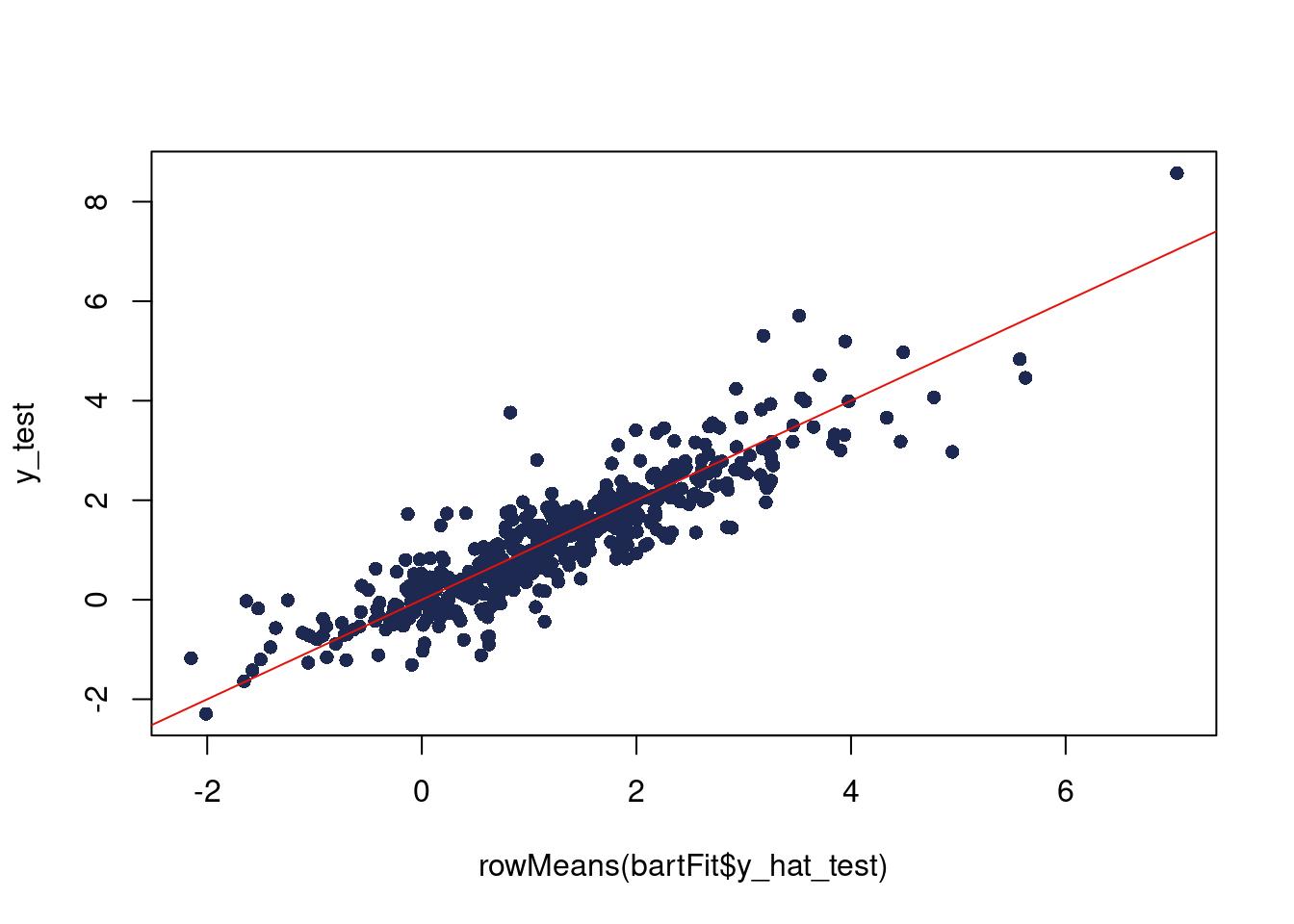
Top: The true relationship between WAR and offensive and defensive rating, from the full dataset. Bottom: The Bayesian optimization predictions compared to the true relation visualized above.

4.5.6 Deeper investigation

A natural question to ask is if the BART surrogate is doing well because of the optimization search, or just because this is an easy, noiseless problem and BART is a good predictor. The following code is meant to illustrate the points that the Bayesian optimization routine selects as where it will learn the most. Compare the selected points to points chosen at random and see if the BART based surrogate optimization is really necessary for these data.

options(warn=-1)
suppressMessages(library(dplyr))
suppressMessages(library(tidyverse))
suppressMessages(library(GGally))
suppressMessages(library(plotly))
suppressMessages(library(NatParksPalettes))
suppressMessages(library(gganimate))
suppressMessages(library(stochtree))



# to store results
num_rep = 20
# start with 15 points randomly selected
design_init = 10
N = 60
set.seed(12024)
RMSE_list = matrix(NA, nrow=N-(design_init-1), ncol = 1)


# consistent X
X_full = X
y = 1000*(nba_ratings$war_reg_season/nba_ratings$mp)

first_guess = sample.int(nrow(X), design_init)

#print(paste0(nba_ratings[first_guess, c('player_name')], '_',
#             nba_ratings[first_guess, c('season')]))



df10 = data.frame(offense = X_train_sub[[1]][,1],
                defense = X_train_sub[[1]][,2],
                war = y_train_sub[[1]])
df20 = data.frame(offense = X_train_sub[[11]][,1],
                  defense = X_train_sub[[11]][,2],
                  war = y_train_sub[[11]])

df40 = data.frame(offense = X_train_sub[[31]][,1],
                  defense = X_train_sub[[31]][,2],
                  war = y_train_sub[[31]])

df60 = data.frame(offense = X_train_sub[[50]][,1],
                  defense = X_train_sub[[50]][,2],
                  war = y_train_sub[[50]])
plot1 = ggplot(df10, aes(offense, defense,
                        z = war)) +
  stat_summary_hex(fun = function(x) quantile(x, 0.50),
                   bins = 16) +

  #geom_point(size=1)+
  geom_tile()+  scale_fill_gradientn(colors=NatParksPalettes::natparks.pals("Acadia"), # Instead, could use MetBrewer::met.brewer('Kandinsky')
                                     limits=c(min(y),
                                              max(y)))+
  ggtitle('First 10 training points (randomly chosen)')+
  xlab('Raptor offense')+ylab('Raptor defense')+
  theme_minimal(base_family = "Roboto Condensed", base_size = 12)+
  theme(plot.title = element_text(hjust = 0.5),
        text = element_text(size = 12))

plot2 = ggplot(df20, aes(offense, defense,
                         z = war)) +
  stat_summary_hex(fun = function(x) quantile(x, 0.50),
                   bins = 16) +

  #geom_point(size=1)+
  geom_tile()+  scale_fill_gradientn(colors=NatParksPalettes::natparks.pals("Acadia"), # Instead, could use MetBrewer::met.brewer('Kandinsky')
                                     limits=c(min(y),
                                              max(y)))+
  ggtitle('First 20 training points')+
  xlab('Raptor offense')+ylab('Raptor defense')+
  theme_minimal(base_family = "Roboto Condensed", base_size = 12)+
  theme(plot.title = element_text(hjust = 0.5),
        text = element_text(size = 12))

plot3 = ggplot(df40, aes(offense, defense,
                 z = war)) +
  stat_summary_hex(fun = function(x) quantile(x, 0.50),
                   bins = 16) +

  #geom_point(size=1)+
  geom_tile()+  scale_fill_gradientn(colors=NatParksPalettes::natparks.pals("Acadia"), # Instead, could use MetBrewer::met.brewer('Kandinsky')
                                     limits=c(min(y),
                                              max(y)))+
  ggtitle('First 40 training points')+
  xlab('Raptor offense')+ylab('Raptor defense')+
  theme_minimal(base_family = "Roboto Condensed", base_size = 12)+
  theme(plot.title = element_text(hjust = 0.5),
        text = element_text(size = 12))
plot4 = ggplot(df60, aes(offense, defense,
                         z = war)) +
  stat_summary_hex(fun = function(x) quantile(x, 0.50),
                   bins = 16) +

  #geom_point(size=1)+
  geom_tile()+  scale_fill_gradientn(colors=NatParksPalettes::natparks.pals("Acadia"), # Instead, could use MetBrewer::met.brewer('Kandinsky')
                                     limits=c(min(y),
                                              max(y)))+
  ggtitle('First 60 training points')+
  xlab('Raptor offense')+ylab('Raptor defense')+
  theme_minimal(base_family = "Roboto Condensed", base_size = 12)+
  theme(plot.title = element_text(hjust = 0.5),
        text = element_text(size = 12))

#ggsave(paste0(here::here(),'/images/NBA_BO_train_set.svg'),
#       ggpubr::ggarrange(plot1,plot2,plot3,plot4, nrow=2,ncol=2,
#                         common.legend=T, legend='right'),
#        height=10, width=14)


#train_size = seq(from=1,to=100, by=5)
train_size = seq(from=1, to=(N-design_init))
preds = unlist(lapply(train_size,
                      function(i)rowMeans(BART_fit[[i]])))
iteration = unlist(lapply(train_size+10, function(i)
  rep(i, nrow(X))))
df2 = data.frame(pred = preds, box_off=rep(X_train[,1],
                                           length(train_size)),
                 box_def=rep(X[,2],length(train_size)),
                 iteration=iteration)



ggpubr::ggarrange(plot1,plot2,plot3,plot4, nrow=2,ncol=2,
                        common.legend=T, legend='right')

4.5.7 Generalize Bayesian optimization

The two examples above both consisted of “constant” (homoskedastic) error. In real life, this is less likely. If we think that the error term might vary with \(\mathbf{x}\), then we should model \(\sigma^2(\mathbf{x})\). We’ll discuss how to do this in more detail in chapter 8, but for now study the code below for a “heteroskedastic” version of the optimization algorithm. The main three lines that change are:

yhats_train <- bart_model_warmstart$y_hat_train[, num_burnin:num_mcmc] + bart_model_warmstart$sigma_x_hat_train[,num_burnin:num_mcmc]*rnorm(nrow(X_train)*(num_mcmc-num_burnin))

yhats_test <- bart_model_warmstart$y_hat_test[, num_burnin:num_mcmc] + bart_model_warmstart$sigma_x_hat_test[,num_burnin:num_mcmc]*rnorm(nrow(X_test)*(num_mcmc-num_burnin))

and

EI = sapply(1:length(new_X), function(j) (1/num_mcmc)sum(sapply(1:num_mcmc, function(i) max((bart_model_warmstart$y_hat_test[j,i]+bart_model_warmstart$sigma_x_hat_test[j,i]*rnorm(1)-f_max),0))))

This is probably a bad idea, as it is hard enough to learn patterns in the variance term as is, let alone with such limited data.

options(warn=-1)
suppressMessages(library(dplyr))
suppressMessages(library(tidyverse)) 
suppressMessages(library(GGally))
suppressMessages(library(plotly))
suppressMessages(library(NatParksPalettes))
suppressMessages(library(gganimate))
suppressMessages(library(stochtree))


RMSE <- function(m, o){
  sqrt(mean((m - o)^2))
}
nba_ratings = read.csv(paste0(here::here(), "/data/modern_RAPTOR_by_player.csv"))
#nba_ratings = read.csv('https://raw.githubusercontent.com/fivethirtyeight/data/refs/heads/master/nba-raptor/modern_RAPTOR_by_player.csv')
# Filter out players with less than 1000 minutes played in a season.
nba_ratings  = nba_ratings %>%
  dplyr::filter(mp>1000)


num_gfr <- 10
num_burnin <- 10
num_mcmc <- 100
num_samples <- num_gfr + num_burnin + num_mcmc
X = as.matrix(nba_ratings[,c('raptor_box_offense', 
                             'raptor_box_defense')])
test_set_pct <- 0.2
n_test <- round(test_set_pct*nrow(X))
n_train <- nrow(X) - n_test
test_inds <- sort(sample(1:nrow(X), n_test, replace = FALSE))
train_inds <- (1:nrow(X))[!((1:nrow(X)) %in% test_inds)]
X_train = X[train_inds,]
X_test = X[test_inds,]
y_train = 1000*nba_ratings$war_reg_season[train_inds]/nba_ratings$mp[train_inds]
y_test = 1000*nba_ratings$war_reg_season[test_inds]/nba_ratings$mp[test_inds]

num_gfr <- 20
num_burnin <- 0
num_mcmc <- 100
num_samples <- num_gfr + num_burnin + num_mcmc
general_params <- list(sample_sigma2_global = F, verbose=F,
                       num_chains=1, keep_every=1)
mean_forest_params <- list(sample_sigma2_leaf = T, num_trees = 50,
                           alpha = 0.95, beta = 2,
                           min_samples_leaf=1, sigma2_init=1e-1,
                             sigma2_leaf_shape = 6, sigma2_leaf_scale = 0.5)
variance_forest_params <- list(num_trees = 5, alpha = 0.95,
                               beta = 2, min_samples_leaf = 1)




# to store results
num_rep = 20
# start with 10 points randomly selected
design_init = 10
N = 60
set.seed(12024)
RMSE_list = matrix(NA, nrow=N-(design_init-1), ncol = 1)


# consistent X
X_full = X
y = 1000*(nba_ratings$war_reg_season/nba_ratings$mp)

first_guess = sample.int(nrow(X), design_init)

print(paste0(nba_ratings[first_guess, c('player_name')], '_',
             nba_ratings[first_guess, c('season')]))
# For plotting purposes
BART_fit = c()
next_step = c()
X_train_sub = c()
y_train_sub = c()

for (k in 1:(N-design_init)){

  # remove these X's
  new_X = setdiff(seq(from=1, to=nrow(X)), first_guess)
  # your initial X's
  X_train = as.matrix(X[first_guess,])
  X_test = X_full#as.matrix(X[new_X,])
  y_train = y[first_guess]
  y_test = y#[new_X]
  
  
  
  bart_model_warmstart <- stochtree::bart(X_train= X_train,
                           y_train = y_train,
                           X_test = X_test,
                           num_gfr = num_gfr, num_burnin = num_burnin, #alpha=0.995, beta=1.25,
                           num_mcmc = num_mcmc, 
                           mean_forest_params = mean_forest_params, 
                          variance_forest_params = variance_forest_params,

                           general_params = general_params)
  
  yhats_train <- bart_model_warmstart$y_hat_train[, num_burnin:num_mcmc] + bart_model_warmstart$sigma_x_hat_train[,num_burnin:num_mcmc]*rnorm(nrow(X_train)*(num_mcmc-num_burnin))
  yhats_test <- bart_model_warmstart$y_hat_test[, num_burnin:num_mcmc] + bart_model_warmstart$sigma_x_hat_test[,num_burnin:num_mcmc]*rnorm(nrow(X_test)*(num_mcmc-num_burnin))
  # the maximum of f up until now
  f_max = max(rowMeans(yhats_train))
  EI = sapply(1:length(new_X), function(j) (1/num_mcmc)*sum(sapply(1:num_mcmc, function(i)
    max((bart_model_warmstart$y_hat_test[j,i]+bart_model_warmstart$sigma_x_hat_test[j,i]*rnorm(1)-f_max),0))))
  
  most_improved = new_X[which(EI==max(EI))]
  if(length(most_improved) > 1){
    most_improved <- sample(most_improved, 1)
  }
  first_guess = c(first_guess, most_improved[1])
  RMSE_list[k, 1] = RMSE(rowMeans(bart_model_warmstart$y_hat_test), y_test)
  BART_fit[[k]] = (yhats_test)
  next_step[[k]] = X_test[most_improved,]
  X_train_sub[[k]] = X_train
  y_train_sub[[k]] = y_train
}


#train_size = seq(from=1,to=100, by=5)
train_size = seq(from=1, to=(N-design_init))
preds = unlist(lapply(train_size, 
                      function(i)rowMeans(BART_fit[[i]])))
iteration = unlist(lapply(train_size+10, function(i)
  rep(i, nrow(X))))
df2 = data.frame(pred = preds, box_off=rep(X[,1],length(train_size)), 
                 box_def=rep(X[,2],length(train_size)), iteration=iteration)

a2 = ggplot(df2, aes(box_off, box_def, z= pred)) + 
  transition_time(
    as.integer(iteration)
  ) +
  stat_summary_hex(fun = function(x) quantile(x, 0.50), 
                   bins = 16) +
  
  #geom_point(size=3.25)+
  scale_fill_gradientn(colors=NatParksPalettes::natparks.pals("Acadia"), # Instead, could use MetBrewer::met.brewer('Kandinsky')
                       limits=c(min(y), 
                                max(y)))+
  labs(title = 'Training size: {frame_time}')+ 
  xlab('Raptor offensive rating')+ylab('Raptor defensive rating')+
  #ggtitle(paste0('Training size = ',design_init))+
  theme_minimal()+
  theme(plot.title = element_text(hjust = 0.5), 
        text = element_text(size = 16))

#a3 <- animate(a2, renderer = ffmpeg_renderer(), width = 700, height = 500)#, options(gganimate.dev_args = list(bg = 'transparent')))
#anim_save(paste0(here::here(),'/images/NBA_BO_anim_het.mp4'), a3)

Assignment **BONUS** (4.3)

1. Traditionally, the Bayesian surrogate people use for Bayesian optimization is a Gaussian process (GP). This is probably due to convenience and inertia. People were taught GP’s, they tend to work well, and have some nice features. They also require a lot of fine-tuning and are difficult to model in practice. We will learn more about GP’s in chapter 8, but if you come back and complete this assignment, you will get bonus points!

---

2. Compare on the 1-d Monte Carlo simulation the BART surrogate and the GP surrogate. Perform \(MC\) repetitions of the Monte Carlo simulations.

---

3. The natural question to ask is if following the uncertainty given from BART and the expected utility criterion is leading us to better regions of the 2-D offense/defense “design space” sooner or if BART is just a really good surrogate (particularly for this easy, noiseless example). Instead of using the expected improvement criteria for the next sampled point in your design matrix, randomly sample a point and see how quickly BART recovers a good approximation of the true output.

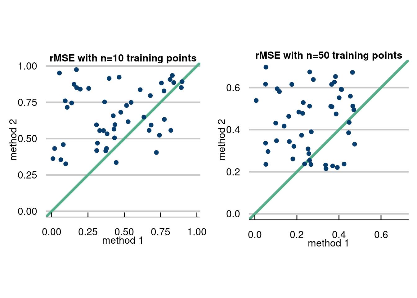
To help with this assignment, here are some vizualizations we like for comparing methods. The first is a general purpose method, while the second is a little more bespoke for this problem.

The first method is a way to visualize when you have ran multiple experiments and had an evaluation metric for each experiment, like the root mean squared error. The idea is to plot the RMSE for method 2 vs method 1 for each experiment and compare which are better. We will show how with a simulated data example below.

The data for the hypothetical RMSE’s are uniform number drawn for each fake method. One of the methods has a higher lower bound and higher upper bound, to visualize that the other method will usually be better (if you’re bored, you can calculate the probability of this). If the data are above the green central bisecting line, then method 1 is better for that Monte Carlo repetition. If it is below, method 2 is better.

list(warn=-1)

$warn
[1] -1

suppressMessages(library(dplyr))
suppressMessages(library(tidyverse))
suppressMessages(library(ggthemes))
MC = 50
BO_10 = data.frame(method1=runif(n=MC, min=0, max=0.9), method2=runif(n=MC,min=0.3,max=1))%>%
  ggplot( aes(x = method1, y=method2)) +
   geom_abline(color='#55AD89', lwd=1.5)+
  geom_point( color='#073d6d', size=2) +
  labs(x = 'method 1', y ='method 2') +
    tune::coord_obs_pred()+

  #scale_fill_manual(values=natparks.pals("Acadia",4))+
  theme_economist_white(gray_bg=F, base_family="ITC Officina Sans") +
  ggtitle('rMSE with n=10 training points')+
  theme(plot.title=element_text(hjust=0.5, size=12))+
  theme(text = element_text(size=12))+
  scale_fill_economist(name=NULL)
BO_50 = 
  data.frame(method1=runif(n=MC, min=0, max=0.5), method2=runif(MC, min=0.2, max=0.7))%>%
  ggplot( aes(x = method1, y=method2)) +
   geom_abline(color='#55AD89', lwd=1.5)+
  geom_point( color='#073d6d', size=2) +
  labs(x = 'method 1', y ='method 2') +
    tune::coord_obs_pred()+

  #scale_fill_manual(values=natparks.pals("Acadia",4))+
  theme_economist_white(gray_bg=F, base_family="ITC Officina Sans") +
  ggtitle('rMSE with n=50 training points')+
  theme(plot.title=element_text(hjust=0.5, size=12))+
  theme(text = element_text(size=12))+
  scale_fill_economist(name=NULL)
gridExtra::grid.arrange(BO_10, BO_50, nrow=1)

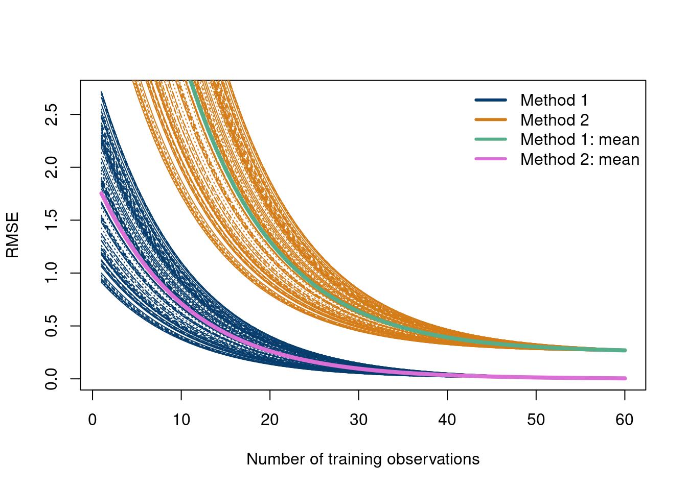
How about looking at the RMSE for different training sizes comparing all \(MC\) Monte Carlo experiments. The data are simulated, but are meant to represent exponentially decreasing RMSE values.

options(warn=-1)

n = 100
t = 60
time = seq(from=1, to=t, length.out=t)
mult = runif(n, 1, 3)
# simulate "sine"half-life" curves with noise and amplitudes "mult"
data = matrix(NA, nrow=t, ncol=n)
data2 = matrix(NA, nrow=t, ncol=n)
for (i in 1:n){
  data[,i] = mult[i]*exp(-time/10)
  data2[,i] = 4*mult[i]*exp(-time/10)+0.25
}

matplot(data, type='l', col='#073d6d', lwd=1, ylab='RMSE', xlab='Number of training observations')
matpoints(data2, type='l', col='#d47c17',lwd=1)
matpoints(rowMeans(data2), type='l', lwd=4, col='#55AD89')
matpoints(rowMeans(data), type='l', col='#Da70D6', lwd=4)
legend("topright", c("Method 1", "Method 2", "Method 1: mean", "Method 2: mean"), col=c('#073d6d', '#d47c17','#55AD89', '#Da70D6'), lty=c(1,1,1,1),bty="n", lwd=c(3,3,3,3))

4.6 Multi-objective optimization

4.6.1 The Pareto front

Agnihotri, Apoorv, and Nipun Batra. 2020. “Exploring Bayesian Optimization.” Distill 5 (5): e26.

Carvalho, Carlos M, Edward I George, P Richard Hahn, and Robert E McCulloch. 2021. “Variable Selection and Interaction Detection with Bayesian Additive Regression Trees.” In Handbook of Bayesian Variable Selection, 395–414. Chapman; Hall/CRC.

Chipman, Hugh A and, Edward I George, and Robert E McCulloch. 2012. “BART: Bayesian Additive Regression Trees.” Annals of Applied Statistics 6 (1): 266–98.

Chipman, Hugh, Pritam Ranjan, and Weiwei Wang. 2012. “Sequential Design for Computer Experiments with a Flexible Bayesian Additive Model.” Canadian Journal of Statistics 40 (4): 663–78.

Gramacy, Robert B. 2020. Surrogates: Gaussian Process Modeling, Design, and Optimization for the Applied Sciences. Chapman; Hall/CRC.

Heiss, Andrew. 2023. “How to Make Fancy Road Trip Maps with R and OpenStreetMap.” June 1, 2023. https://doi.org/10.59350/rgwda-0tv16.

Lei, Bowen, Tanner Quinn Kirk, Anirban Bhattacharya, Debdeep Pati, Xiaoning Qian, Raymundo Arroyave, and Bani K Mallick. 2021. “Bayesian Optimization with Adaptive Surrogate Models for Automated Experimental Design.” Npj Computational Materials 7 (1): 194.

McElreath, Richard. 2018. Statistical Rethinking: A Bayesian Course with Examples in r and Stan. Chapman; Hall/CRC.

Newman, Mark. 2013. “Computational Physics.” (No Title).

Silver, Nate. 2012. The Signal and the Noise: Why so Many Predictions Fail-but Some Don’t. Penguin.