In this chapter, we will focus more on different models describing multiple variables. This includes joint outcome models, models about the dependency between multiple inputs, and models using the dependency of different variables to fill in missing data. We will discuss different measures of dependency between variables as well as ways to generally describe similarity between units.
11.1 A naive approach to modeling multiple outcomes
The following data describe US presidential election modeling. The data include the results from the 2012, 2016, and 2020 elections, the polling averages from 2016 and 2020 (from fivethirtyeight’s polling average), and some demographic data from the 2017 census. We will model the democratic candidate’s vote share and republican candidate’s vote share in 2020 separately, the simplest way of modeling joint outcomes. We will also show some heuristics for how to see if this simple approach is sufficient, or if we need to think harder.
This problem is hard for a variety of reasons. Obviously, the republican and democratic vote shares depend on each other, so predicting them separately is a big simplification. Even then, we are predicting 50 states where there are plausibly correlated errors (if we miss Michigan, we will probably miss similarly in Wisconsin). The trees in BART tend to do a good job grouping together similar observations, but we will try and help in this regard by adding demographic data and indicators for the region of the country. A more formal approach would be a hierarchical model, where a random effect term should help capture variation common across the countries but also unique to different regions of the country. See the assignment for your task on this.
The data were downloaded and cleaned from fivethirtyeight’s polling database. We downloaded the “presidential general election polling average” file and cleaned it using the following script, which is not run because the data was a little too large to upload to the github folder, so we recommend downloading it locally then running this script if interested.
print(paste0('The RMSE for democrats is: ',round(RMSE(rowMeans(bart_fit_dem$y_hat_test), merged3$dem_perc_2020),2)))
[1] "The RMSE for democrats is: 4.52"
Click here for full code
print(paste0('The RMSE for republicans is: ', round(RMSE(rowMeans(bart_fit_rep$y_hat_test), merged3$rep_perc_2020),2)))
[1] "The RMSE for republicans is: 2.76"
Click here for full code
print(paste0('The overall RMSE is: ', round(RMSE((rowMeans(bart_fit_dem$y_hat_test)-rowMeans(bart_fit_rep$y_hat_test)), (merged3$dem_perc_2020-merged3$rep_perc_2020)),2)))
[1] "The overall RMSE is: 5.17"
So those fits are … okay … The wide credible intervals are not particularly comforting to see. Let’s dig a bit deeper into the residuals of each model.
data('fifty_states')grid.arrange(df %>%mutate(state =tolower(merged3$state))%>%group_by(state)%>%# map points to the fifty_states shape dataggplot(aes(map_id=state))+geom_map(aes(fill = dem_fit-dem_actual),color='black',lwd=0.7, map = fifty_states) +expand_limits(x = fifty_states$long, y = fifty_states$lat) +coord_map() +scale_x_continuous(breaks =NULL) +scale_y_continuous(breaks =NULL) +labs(x ="", y ="") +ggtitle('Fit of democrat percent minus actual democrat %')+#scale_fill_gradient2scale_fill_gradient(low ="#073d6d", high='#f8f9fa')+theme(legend.position ="bottom",plot.title=element_text(hjust=0.5, size=12),panel.background =element_blank(),text=element_text(size=14)),df %>%mutate(state =tolower(merged3$state))%>%group_by(state)%>%# map points to the fifty_states shape dataggplot(aes(map_id=state))+geom_map(aes(fill = rep_fit-rep_actual),color='black',lwd=0.7, map = fifty_states) +expand_limits(x = fifty_states$long, y = fifty_states$lat) +coord_map() +scale_x_continuous(breaks =NULL) +scale_y_continuous(breaks =NULL) +labs(x ="", y ="") +ggtitle('Fit of republican percent minus actual republican %')+#scale_fill_gradient2scale_fill_gradient(low ="#073d6d", high='#f8f9fa')+theme(legend.position ="bottom",plot.title=element_text(hjust=0.5, size=12),panel.background =element_blank(),text=element_text(size=14)), nrow=1)
Click here for full code
# Instead of including the region as a feature, one could treat this as a random effect modeling# exercise, follow this example:# https://stochastictree.github.io/stochtree-r/articles/CustomSamplingRoutine.html#demo-3-supervised-learning-with-additive-multi-component-random-effects
We should see a pattern in the first plot. If a democratic candidate under-performs, it is likely because the republican candidate took some of their votes. So we should see a pattern there, which we do not. Given that we fit the models independently, this is not super surprising.
As for the second plot, do we see any spatial correlations?
Assignment (11.1)
One of the major complaints a more seasoned forecaster would have with the modeling approach we just took is the lack of sufficient data. We can certainly do better. Additional attributes could include economic indicators, polling trends, approval ratings, more historical data, and other things. Additionally, engineering cool features out of these attributes could yield far better predictive accuracy. So, that is your task. Find more data and create interesting features out of them to improve the inputs to the BART model. Make a forecast for 2024. You can include every variable above including 2012, 2016, and 2020 results. We trained on 2016 to predict on 2020 as a proof of concept, but you may as well use all the data available.
We discussed how there seems to be some correlation between the residuals of the republican and democratic vote share predictive models. This is indicative of some dependence on the errors, meaning we need to think a little more carefully about how to model the outcomes jointly. This is somewhere where a software like PyTorch comes in handy, as joint outcome modeling with neural networks is well established and easier to implement. However, neural networks, in our experience, do not tend to predict this type of tabular data well out of sample, limiting its utility as a forecasting tool here.
In the above example, we saw a clear bias in the polling data, particularly in 2020, where the republican candidates vote share seemed to be systematically underestimated. The polls margin of error describes a statistical generalization error between a sample and a population; this error seems to be more fundamental and representative of a bias in the population estimate. One thing to consider would be a error in variable model. What we will suggest is more crude and janky. Instead of running one BART model with the polling average, we will run many on separate posterior draws of the polling averages estimated from a Bayesian model. This procedure isn’t really Bayesian anymore, as we are now running the model on hypothetical new \(\mathbf{x}\) (covariates), so we are just using BART as a strong point estimate model. The procedure also introduces extra variance into the forecasting process, so it is probably not the best idea, but we are suggesting it more as an exploratory exercise.
If we are to proceed down this route, we want to make sure to make sure simulate polling values correlate across states. For example, a change in a Wisconsin polling value from the reference (the average from 538) should also lead to a similar change in Michigan. Since we have multiple polls from every state, we could generate draws from a multivariate normal (with one dimension per state) that represent the correlations between states. This is similar to the methods we learned about with the multivariate normal, as well as “copula” modeling we will learn about later.
An alternative approach would be to fit a hierarchical model, similar to the rat-tumor data, would be to shrink the polling estimates for a state to a similar value of nearby states (where nearby could be defined by region or some statistical clustering technique). Adapting the code from the rat-tumor data should make this fairly straightforward. Caveat, this approach still isn’t modeling the joint outcomes of the polls, and would require doing the model for just democratic, or just republican polls, or maybe the margin between them.
11.1.1 Creating synthetic polling data (probably a bad idea)
We will look at 5 swing states from 2020’s polling data: Arizona, Georgia, Michigan, Pennsylvania, and Wisconsin. We will assume there is -3 bias against republicans in these polls (which was borne out to be roughly true, but lets treat this as a hunch).We will also generate from the multivariate student t distribution, which allows for more outlier situations due to the heavier tails, generating with the suggestion from this excellent stackoverflow link. Of course, we could also run these simulations with each observed poll as a different input, which would add less artificial variance than a modeling approach would. However, how to vary the polls so that states vary together is potentially tricky.
Let’s get to work on creating the synthetic data. Again, maybe not the best idea, but since we are trying to forecast, statistical rigor and inference is not necessarily our goal. Ideally, you want your forecast to generalize, but if you just want a good prediction for a certain election (where you have strong priors), maybe not the worst idea.
Registered S3 method overwritten by 'GGally':
  method from
  +.gg   ggplot2
Click here for full code
suppressMessages(plot_df_norm)
`stat_bin()` using `bins = 30`. Pick better value with `binwidth`.
`stat_bin()` using `bins = 30`. Pick better value with `binwidth`.
`stat_bin()` using `bins = 30`. Pick better value with `binwidth`.
`stat_bin()` using `bins = 30`. Pick better value with `binwidth`.
`stat_bin()` using `bins = 30`. Pick better value with `binwidth`.
Now, we will simulate synthetic polls from a multivariate student t with 4 degrees of freedom.
`stat_bin()` using `bins = 30`. Pick better value with `binwidth`.
`stat_bin()` using `bins = 30`. Pick better value with `binwidth`.
`stat_bin()` using `bins = 30`. Pick better value with `binwidth`.
`stat_bin()` using `bins = 30`. Pick better value with `binwidth`.
`stat_bin()` using `bins = 30`. Pick better value with `binwidth`.
Again, this is probably a bad idea! See (Goorbergh et al. 2022)link and (Carriero et al. 2024)arxiv link. Both these articles discuss the similar, but different, idea of synthetic oversampling of under-represented classes in your data and how it can bias your results. These papers describe the statistical issues with oversampling the less represented group, and how it can lead you to overestimate their prevalence with your predicted probabilities. The issue with the simulated approach above is that we are imposing too much of our prior knowledge by assuming a directional, systemic bias in the polling averages by state. But, the SMOTE papers are important and seemed like a good place to include them.
11.2 A little more on correlated errors
Generally, in linear regression assumptions we talk about the errors being correlated with a single outcome (so different \(y_i\) ’s have correlated error terms \(\varepsilon_i\)), but here we talk about the errors for multiple variable outcomes being correlated. This is an issue that goes beyond linear regression and we are not necessarily saved by simply using a fancy regression model.
It’s a common misconception that modeling two outcomes is only problem if the outcomes are correlated. There are difficulties in modeling the outcomes jointly to be sure, and explicitly modeling the relationship between the outcomes can improve predictions of both as it incorporates additional information about both outcomes. If the outcomes are functions of one another, then modeling both is essentially just giving us more information which should de-noise the problem. See (Breiman and Friedman 1997). We would want shared information between our two models to help with this. For example, a neural network modeling two outcomes would want to have hidden layers map to both outcomes, to try and ensure the relationship between the variables is captured.
However, a potentially bigger issue can be found in the error terms, particular if . Consider:
In this case, two independent linear regression models should be able to estimate the coefficients on \(y_1\) and \(y_2\) perfectly fine. \(y_1\) and \(y_2\) are certainly correlated, but because the error terms (which we do not see) are independent we are okay in modeling the outcomes separately. Of course, as (Breiman and Friedman 1997) suggest, we may see benefits if we do model them jointly, but more on that later.
Now, consider when the error terms are correlated. These terms aren’t actually observed, so if they are correlated then there will be a dependence between unobserved terms in the \(y_1\) linear regression and \(y_2\) linear regression that we do not model (remember
Where \(\mathbf{I}\) is the identity matrix. In the case of heteroskedastic noise, the diagonals have different values, meaning that for different values of the covariates, the error can change. If there is correlated error, then the non-diagonal terms are non-zero, i.e. \(\varepsilon \text{ call $\mathbf{U}$}\sim N(0, \mathbf{\Sigma})\).
This is related to the concept of seemingly unrelated regression. In that example, two outcomes are not correlated except through their error terms!
Anyways, the following script shows the issue when modeling the different outcomes with independent linear regression models instead of modeling \(\mathbf{\Sigma }\).
The plot above shows when two separate models are okay. The data are generated so that \(\varepsilon_{1}\)and \(\varepsilon_{2}\) are independent. The bottom row shows \(y_1\) is well approximated by \(\hat{y}_1\), and \(y_2\) is well approximated by \(\hat{y}_2\). Additionally, the plot of \(y_2\) vs \(y_1\) in the top left shows the same correlation as the plot of \(\hat{y}_2\) vs \(\hat{y}_1\) in the top right. So each model predicts well and the outcomes are predicted well jointly. Now, we will have a strong correlation factor between the two outcomes error term which induces some dependence between the two outcomes (that we did not see in the previous plot).
The above plots are from a data generating process where \(\varepsilon_{1}\) and \(\varepsilon_{2}\) are strongly correlated (they are drawn from a bivariate normal distribution with \(\rho=0.99\). What do these plots show? We see in the bottom rows that we predict \(y_1\) and \(y_2\) fairly well with our linear regression model. However, in the top right corner, we see that there is a small negative correlation between \(\hat{y}_1\) and \(\hat{y}_2\), whereas in reality \(y_1\) and \(y_2\) have some positive correlation (see the top left corner). So the takeaway is we still estimate the \(\beta\) parameters well with independent models, but our intervals for the parameters will be wrong. In fact, the maximum likelihood estimator for \(\mathbf{B}\) in \(\mathbf{y}=\mathbf{X}\mathbf{B}+\mathbf{U}\)1 is the same as the usual estimator for \(\beta\), meaning fitting two separate regression models won’t change your estimate (see OLS vs GLS). This is evident with the joint distribution of \(Y_1\) and \(Y_2\) being wrong. Now, because the error terms are off, this is why inference will be off and intervals will be incorrect, even with good mean estimates.
1 Where \(y\) is the stacked vector of the multiple outcomes, and \(U\sim \mathcal{N}(0, \mathbf{\Sigma})\) encodes the information that the errors are correlated across outcomes
11.3 BART to the rescue
Even if we use a fancy machine learning method, we are still at risk when modeling outcomes with correlated errors, as we saw with the election forecast2. But now with our additional knowledge, we will show a (sort of) “remedy” that at least handles the correlated function aspect of the problem. A solution is to use a shared forest to model both the outcomes! This does not explicitly do anything about the correlated errors, but it does push the estimates for the democrat and the republican towards their functional relationship. That is, we can improve the individual predictions of the two outcomes, since they are essentially noisy functions of the other, so modeling both concurrently should serve as a regularization mechanism for both the predicted outcomes. That is, we are currently roughly modeling \[
\begin{align}
\text{Biden} = f(\mathbf{x})+\varepsilon_{1}\\
\text{Trump} = 1-f(\mathbf{x})+\varepsilon_{2}
\end{align}
\]since each is a noisy estimate of the other (essentially), then sharing the split locations serves to better utilize the extra information endowed by doubling the sample size in the BART training stage. We are less likely to overfit or chase noise if we have additional information by building trees to fit \(f(\mathbf{x})\) and \(1-f(\mathbf{x})\). This is because even in the absence of correlated errors, if the signals are associated, then sharing information between the model fits amounts to essentially increasing the sample size for each outcome being inferred. This is generally a good thing (computational time aside).
2 There is also, and probably more problematically, spatially correlated error, even if we only cared about 1 outcome. The correlation between republican and democratic vote share is probably reasonably well modeled by predicting democratic percentage and setting republican prediction to 1-democrat prediction, since there are not a ton of third party voters.
Of course, there is still reason to believe the errors are correlated, and \(\varepsilon_{1}\) is not independent of \(\varepsilon_{2}\).
so we’d also like to model the error term in the BART model explicitly.
To model the outcomes jointly, we would like the two outcomes to share leaf node locations (not values) so as to share information between the two models. One way to do this3 is by alternating which outcome a BART forest predicts. Doing so invalidates the procedure as a Bayesian one, as only half the response data (Biden or Trump’s vote share) is used in each step. However, the proposed approach could still useful for this problem, as we jump between predicting Biden and Trump’s vote share using the same covariates and pass the built tree from Biden to Trump and back again for each sweep through the forest. This helps (heuristically at least) share forests between the two response models, which is useful since being wrong about Biden will also likely make us wrong about Trump4. Of course, more care should be taken, to ensure a valid sampler is produced and for a more general purpose methodology. We will use the “shared forest” motivation for the above method to describe a more rigorous and correct approach.
3 Which is problematic as we shall soon see.
4 Overestimating Biden will likely underestimate Trump for example
11.3.1 Revisiting the naive election model
First, note that we saved a version of the cleaned election data (the merged 3 file used for the BART fittings earlier) to save space. The file is called cleaned_election_data.csv.
Now, let’s do the election situation (more) properly! The code below is the “cleaning data code” we will need for our proposed approach.
Before we describe our proposed fix, you have an assignment.
This might a lot of extra work for nothing. Or maybe its not enough work. Either way, its more work for you.
Assignment
Instead of using a shared forest approach, fit the democratic candidates model and make the republican model equal to 1 minus the democrat.
The issue with 1) is that we are not accounting for third party candidates. We also do not model 3rd party candidates in the shared forest approach. Add the third party as a third outcome to the shared forest loop and see if it helps!
A constraint such that republican + democrat is less than 1 occurs in nature. On a practical note, it seems like for different MCMC draws this is violated, and at times pretty badly. Fixing this would likely require bespoke BART model with a custom outcome likelihood (like a truncated normal) and doing that would require a lot of work. Your task is to investigate how badly this constraint is violated and if you can make choices to the hyper-parameters or the feature engineering to help.
11.4 Joint outcome modeling: Take III
We will explore how to use stochtree to predict multiple outcomes simultaneously. We will use election forecasting to highlight the methods described, with several nice customizations added in to address the particular quirks of the applied problem at hand. Stochtree provides a nice vehicle to easily implement these bespoke features.
A motivating approach for modeling joint outcomes that we know to have some correlation can be found in (Breiman and Friedman 1997). They develop the “curds and whey” procedure, a “multivariate shrinking” tool for modeling joint, correlated outcomes (linked here). They find that explicitly accounting for the joint structure of the outcomes offers improved prediction accuracy over separate OLS linear regressions in the case the outcomes are actually correlated and that it does no harm when they are not. The shared forest approach aims to accomplish a similar goal but in the context of a more flexible, non-parametric model.
In the situation where we have multiple outcomes we want to model, we should also take great attention to respect any correlated error terms between the two outcomes. Even if the respective conditional means are predicted well by independent models, this approach will not capture the dependencies in the error terms of the two outcome models. No fancy machine learning method can remedy this without further care. This is related to the concept of seemingly unrelated regression(Zellner 1962). Two outcomes can be correlated potentially only through their correlated error terms! To address the correlation in errors across outcomes, we include a random intercept for each state pair. We also make a significant effort to model spatially correlated errors, which are more of an issue in the election forecast.
11.4.1 Election forecasting revisited
A nice example of jointly correlated outcomes can be found in U.S. presidential election forecast modeling. We have tried to solve this problem twice already, but now tackle it with more rigor.
Since U.S. presidential elections only usually have two major candidates with minimal third party support, we expect the support of the republican and democrat to be linked.
Election modeling also provides a nice example of correlated errors across outcomes as well5. In the above mental model, this means that \(\varepsilon_{1}(\mathbf{x})\) and \(\varepsilon_{2}(\mathbf{x})\) arise from a joint correlation structure. Intuitively, overestimating the democrat will likely underestimate the republican.
5 More pernicious in election modeling are spatially correlated errors. If you over-estimate Biden in Michigan, you are very likely going to over-estimate him in Wisconsin and Pennsylvania. This issue led (in part) to the beef between Andrew Gelman and Nate Silver over how their election models handled this issue.
11.4.2 About the data
The data constituting our design matrix, \(\mathbf{x}\), for the election model include demographics, polling averages, results from the previous election, and regional indicators for states. Demographics are from the U.S. census bureau pulled in 2017. The polling data come from fivethirtyeight aggregations from the day before the 2016 and 2020 elections. The results from the previous election are comprised of the percent of vote share the republican, democrat, and other received in the previous election. In the case of 2016, this means the 2012 election, and for 2020 these data are from the 2016 election. Finally, we have the region code for every state that we include as one-hot encoded columns.
These data are quite limited. For one, we use the same demographic data for each state for 2016 and 2020. We also only report the polling average the day before the election. Trends & variance would be useful metrics to include here as well. We also omit any data on approval ratings or economic conditions. Finally, we only train on the previous election, which is limiting.
Our goal is to predict the vote shares of Biden and Trump in 2020 simultaneously from a model trained on the 2016 election. As we have mentioned, we want to devise a tool that can model the outcomes flexibly in the face of limited data, while also being cognizant of the dependence structure on the two outcomes. In a sense then, this seems like an inspired use of BART. On the other hand, polling has become more and more difficult over the years and turnout is difficult to predict, so hedging your bets on any model for forecasting election results is not wise.
Fit the democratic and republican candidate with separate models. This is a naive first approach and is just that. The two outcomes are connected in a particularly troubling way. The errors in predicting Biden will be correlated with the errors in predicting Trump. If you want just the point estimates for Biden and Trump, then averaging over the posterior for each prediction this will probably give fine predictions6. However comparing the posterior draws to see who “wins” will be problematic, since we are not considering the outcomes simultaneously. Unfortunately, this is a pre-requisite to modeling the uncertainty of the election forecast.
A simple fix for this is to fit the Biden model and then estimate Trump as 1-Biden. This is a good thought and in the case of having only two candidates, be exactly what we want. However, third party candidates vote percentage vary by state. For example, Utah had a fairly serious third party candidate in Evan McMullin in 2016, whereas other states did not. This leads us to think for thoroughly about the problem at hand.
Use the leaf regression formulation in stochtree to our benefit. This link provides derivations for marginal likelihood calculations that enable computation of the BART posterior. This will allow us to share forests between the two outcome models, which can help regularize both models appropriately7. The shared forests are useful here since the outcomes are functions of one another, so we’d expect the same tree structure should be used to partition the data for both outcomes, with the only difference being the actual values in the leaves and which outcome they belong to. This allows us to “pair” the outcomes by modeling their joint “functional” dependence.
6 With careful prior choices and modeling decisions (such as modeling the error term to incorporate heteroskedasticity)
7 Since the outcomes functions are pretty strongly related, then building trees to accomodate both outcomes should improve the fit of each.
The general idea for creating shared forests presented here depends on two concepts: data augmentation and leaf regression. The first helps ensure the splits are consistent between the two outcomes and the second ensures we fit the correct level for each outcome in the leaves.
The adapted machinery begins by stacking our design matrix and our two outcomes, \(Y_{\text{Biden}}\) and \(Y_{\text{Trump}}\). That is:
Where Biden and Trump will have the same heteroskedastic error term \(\varepsilon(\mathbf{x})\) and there is a state level random effect, \(\gamma\). How does this formulation help us? By ensuring that both the outcomes have the same design matrix, we guarantee that each outcome shares the same splits and tree structure. As we discussed, this is a feature we want in order to share information between outcomes. Building the trees to fit Biden and Trump concurrently serves to regularize both estimates, since Biden’s vote share is roughly 1-Trump’s, and vice versa. So the shared forests serve the primary purpose of improving estimates of the conditional mean for each outcome by incorporating both outcomes (which are functionally related). The random intercept is there to account for correlations in the error terms between the outcomes and the heteroskedastic error term accounts for the potential that there is a different variance for the error across different states.
To build intuition for why the random effect can help with modeling correlated errors, consider the following simulation:
The random effect “eats into” the error term in a sense. The groups, in this case the observations across the two outcomes, have the same term added to their error distributions. This means that the groups will have their overall error be correlated, depending on the strength of the random intercept.
Where does the leaf regression come into play? Without the leaf regression, the same splits on the \(\mathbf{x}'\)s will be forced to predict on two different outcomes, likely predicting the mean of the two outcomes (which should be around 50% of the vote share). By including a different basis for each outcome in the leaves, we are essentially running two “intercept” regressions for the two different outcomes. This can be stated mathematically as (looking at just the level prediction within a leaf of a tree):
With the data augmentation plus the bespoke basis in the leaf nodes of the trees in the BART forest, we have developed a base procedure for multiple outcome regression. Some additional care is desirable however.
Given that we are training only on 2016 presidential election data, we only have 50 data points! This guides our decision to press for more regularization. This means a higher \(\beta\) and less trees than the default.
Additionally, we are only looking at the averages of polling data from the day before the election. It is reasonable that we can expect more certainty in swing state polling, since we are averaging over many polls, whereas a small, reliably blue state like Vermont likely had very few polls (which are also likely to be lower quality). Therefore, modeling heteroskedasticity presents a prudent choice. This is done by modeling the variance term through the log-linear BART model of (Murray 2021).
Spatially correlated error have doomed many election forecasts in the past. This is something we also consider. By including dummy variables for the region of the United States a geographic state resides in. If you would like to use the region as a random effect with the regions as group, pass the group_id_region variable as the argument to rfx_group_id_train and rfx_group_id_test in the code below. Since we have included the regions as covariates into our design matrix, as well as demographic data on each state, we have faith that the base BART model will capture effects by partitioning similar states into the same leaf nodes.
A random effects model (see the high-level stochtree interface), is used to help account for correlated errors between the outcomes. This approach is similar to the work of (Tan, Flannagan, and Elliott 2018), who add a random intercept to the standard BART model to predict whether a driver would stop at an intersection, with multiple outcomes per driver. We include a random effect where the “groups” correspond to the states. This is an attempt to model the correlated error we discussed earlier. This argument is added from the rfx_basis_train , rfx_basis_test, group_id_train, and group_id_test lines in the stochtree::bart() arguments. In the code below, a random intercept model for the states is implemented. The states are paired accross outcomes, so each state has the same intercept (drawn anew for each MCMC iteration) added to the prediction for both outcomes. Conveniently, this is also handled in the high-level stochtree interface, so no custom samplers are required!
To summarize, this problem actually provides a nice exploration of many of the features stochtree provides. We utilize multivariate leaf regression, a random effect intercept model (Tan, Flannagan, and Elliott 2018), the XBART warmstart method (He and Hahn 2023), and model heteroskedasticity in the variance term (Murray 2021). These “additions” to the standard BART model are extremely useful for this application, and can be implemented fairly easily in stochtree.
11.4.5 Data analysis
The following code chunk will “clean” the data a little (it was mostly already pre-processed). The only painstaking thing here is defining the group identifiers for the region random effect. Since the pre-cleaned data already one-hot encoded the design matrix, we have to convert the regions back into their single column form. So it goes.
As for setting BART prior and hyper-parameter priors, we encourage small trees to regularize, which feels like a must given the small data sizes and that we know that elections do not vary super wildly from the polls (depending on who you ask) and the previous cycle.
Let’s examine the posterior distribution for each outcome. Visualizing this can be done in many ways. qm2 in the previous code chunk will give 95% posterior intervals for the predictions of every state for each outcome. For a more thorough visual, we will zero in on Arizona. The blue histogram is for Biden and the red for Trump.
There does appear to be some auto-correlation in these draws if we follow the same colors. This is indicative of some potential poor mixing in specific independent MCMC chains. This was our motivation for running 10 independent chains, each beginning at one of the
“grow from root” XBART trees that initialize the warmstart (He and Hahn 2023), (Krantsevich, He, and Hahn 2023). The idea is that each chain will explore different regions of the posterior space, so even though the individual forests from each don’t necessarily mix well, aggregating them might help mitigate this. Given the small sample size and the fact that the chains are parallelizable since they are independent, this is not a huge computational strain.
Let’s see how our win probabilities8 match up with what happened:
8 Calculated by taking the pairwise difference of the posterior probabilities across MCMC draws and assigning the higher predicted vote share the victory. Dividing the number of wins by total MCMC draws.
Forecast: forecasted Biden minus Trump margin, Actual: actual Biden minus Trump margin
* Error for poll favoring Biden
† Intervals from 2.5 and 97.5% quantiles of BART posterior differences
Let’s examine the residuals of our two outcomes. As discussed above, we expect Trump’s vote share to be roughly 1 - Biden’s. We will plot this below to inspect. An additional feature in this plot is to color code every state by how much the polls underestimated Trump’s support9.
9 Trump’s support was famously under represented in polls in 2016 and even more so in 2020.
Another nice thing to look at is a confusion matrix:
Click here for full code
confusion_table =table(Biden_pred_win=win_probs$`Biden win probability`>win_probs$`Trump win probability`, Biden_actual_win=merged3$dem_perc_2020>merged3$rep_perc_2020)cm =confusionMatrix(confusion_table)# Convert to data frame for ggplotcm_df <-as.data.frame(cm$table) cm_df$Biden_pred_win =c('Biden pred loss', 'Biden pred win', 'Biden pred loss', 'Biden pred win')cm_df$Biden_actual_win =c('Biden actual loss', 'Biden actual loss', 'Biden actual win', 'Biden actual win')ggplot(cm_df, aes(x = Biden_pred_win, y = Biden_actual_win, fill = Freq, label=Freq)) +geom_tile() +xlab('')+ylab('')+scale_fill_gradient(low=c("#6f95d2"), high="#012296") +geom_text(color='white', size=8)+theme_minimal(base_family ="Roboto Condensed", base_size =22) +theme(plot.title=element_text(hjust=0.5, size=12),legend.position="none")
11.4.6 Summary
The model performance is actually excellent, despite the limited data. This was a tricky problem in a lot of ways. We had two outcomes that depend on another. Each outcome is a noisy realization of a, complex combination (but probably not enormously complex) of the input data. The data size to train on are limited. These considerations facilitate the need for a regularized but flexible regression tool.
We are also very concerned with proper quantification of our uncertainty, particularly in the error terms in our model. The “learnable signal” certainly depends on state, due to discrepancies in polling by state, meaning we can expect the error term to depend on covariates, i.e. heteroskedasticity is present. This complicates a more straightforward modeling of the error term in a standard model. Additionally, errors in predicting Biden should affect errors about Trump (over-estimating one likely underestimates the other). Finally, our uncertainty in different states should raise or lower together. Error in Michigan will likely be correlated with the error in Wisconsin. These considerations make a more standard modeling approach difficult, if not entirely unreliable. Luckily, stochtree allows all these modifications to be made with minimal coding implementation.
Here are some pros of the model we described above, with a couple limitations to address below.
(+) The outcomes are strongly linked and devising a shared forest regime helps incorporate that extra information and regularize both estimates better.
(+) There are likely spatially correlated errors and the random effect helps.
(+) Error is also probably heteroskedastic, taken care of.
(+) Extra regularization due to small sample sizesand our prior knowledge of the intense polarization in 2020. We found it wise to not really entertain extreme scenarios a priori. BART provides a natural engine for strong regularization, while also remaining flexible enough to signals in the data to override this prior if need be.
(+) Stochtree specific: The warmstart approach (that is the default) and running multiple chains greatly helped the mixing. Having both these features available with a single line of code is a great boon to applied statisticians and data modelers
(-) Because of the small sample size, the predictions are pretty sensitive to hyper-parameter choices and how long we run the sampler. The first is part of applied modeling: we cannot realistically except off the shelf choices to always work really well (although they do work pretty well in this example). The second is aided by running more chains, which was easily implemented in stochtree and is easily parallelizable if you have multiple cores!
(-) The outcomes are constrained to sum to less than 1. We punt on accounting for this explicitly at the moment, but it would be a nice addition to this applied problem.Copulas
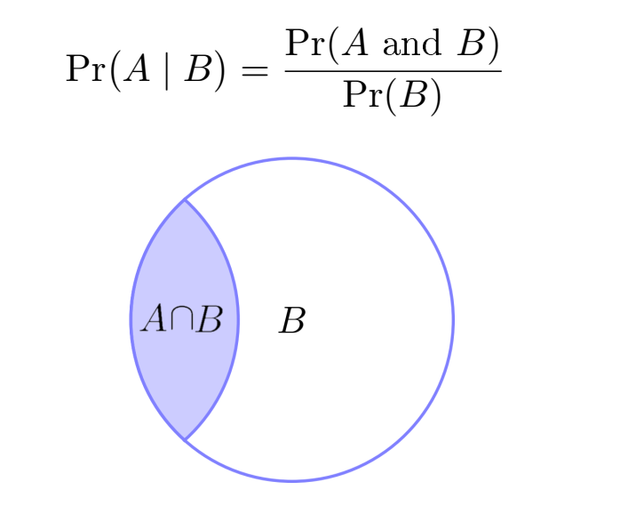
This section will serve as a friendly introduction to copula modeling. Copulas are a natural extension to our previous topics, as they provide a really nice way to separate “joint distributions” (everything together) and “marginal distributions” (everything on its own in the absence of the others). Marginal and conditional are sometimes confused. A marginal distribution is the distribution of a variable absent the other variables, and conditional is the distribution given other variables. The confusion comes because to find a marginal distribution, you add all the possible values the other variables could be and average their contributions. That is, you take a weighted sum of your variable conditional on the others weighted by the distribution of those other variables.
The following are a few nice resources to introduce copulas.
Here is our attempt to explain them in an intuitive way. The copula of random variables \(X_1, X_2, \ldots, X_p\) is given by
\(\Pr(U_1<u_1, U_2<u_2, U_3<u_3,...)\)
where the \(U_i\) are uniform random variables. Wait what the ****, where did the uniforms come from? From the probability integral transform, the cdfs of every \(X_i\), \(F_i(x)=\Pr(X_i< x)\) is itself distributed uniformly. Let’s check this out in code:
Click here for full code
n =5000z <-rnorm(n)hist(z, col='#073d6d', main='Normal distribution')
Click here for full code
hist(pnorm(z), col='#55AD89', main='Distribution of normal CDF')
hist(pgamma(gam,1,1), col='#55AD89', main='Distribution of gamma CDF')
What a copula is then is just the joint distribution of the cumulative distribution function (cdfs) of a bunch of random variables. Conveniently,\(X<F^{-1}(u)\), will also yield a uniform distribution (because \(F^{-1}(u)\) will return the original distribution). This means we can write the copula (equivalently as before) as
We can then choose the CDF to model the resultant joint distribution after any marginal transformations we make. And the choice of the CDF function (whether it be a multivariate normal, which doesn’t model tail dependence, or multivariate t distribution or something else) encode dependencies in different ways.
About those marginals. Because \(F_x(x)=u\), then it is also true that \(x=F^{-1}(u)\). This is why we are permitted to transform the now uniform marginal random variables to any distribution we would like (while also maintaining the joint dependencies of the variables \(X_1, X_2, \ldots, X_p\)). To reiterate, this means we can model the marginal distribution of the \(X_i\)’s independently of one another (meaning we can model each \(X_i\) with a different probability distribution) any way we like. Doing so means the random variables are transformed, but just marginally. Any further transformations to the marginals of the Copula does not change the dependence structure because the CDF of any distribution is uniform, so the inverse of a distribution applied to the uniform will give the correct marginal distribution we want.
11.5.1 NBA data
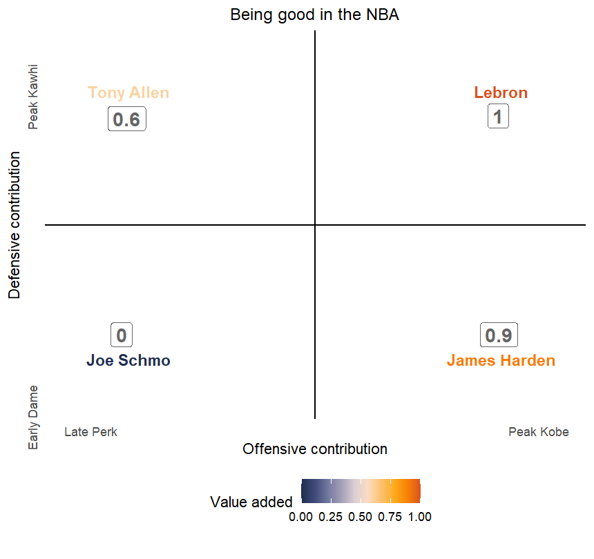
Players who do not play good defense or offense won’t be in the NBA. We hypothesize that elite offensive players are more valuable than elite defensive players.
The following data example should help clarify some of the more confusing aspects of the previous simulation based approach. The data are from the fivethirtyeight github repo, which contains many excellent datasets. Specifically, we look at the “nba-raptor” dataset, which consists of data from the Raptor forecasting tool fivethirtyeight used to use (fivethirtyeight player ratings), which itself is a successor to the popular Carmelo projections model, both of which are now unfortunately defunct.
The data we will analyze are the offensive score, defensive score, and WAR (wins above replacement, an overall value metric) statistics given in the RAPTOR dataset.
Click here for full code
options(warn=-1)suppressMessages(library(dplyr))suppressMessages(library(tidyverse)) suppressMessages(library(GGally))suppressMessages(library(plotly))nba_ratings =read.csv(paste0(here::here(), "/data/modern_RAPTOR_by_player.csv"))# Filter out players with less than 200 minutes played in a season.nba_ratings = nba_ratings %>% dplyr::filter(mp>250)X =data.frame(nba_ratings$raptor_box_offense, nba_ratings$raptor_box_defense, nba_ratings$war_reg_season)X = X %>%mutate_if(is.numeric, round, digits=3)colnames(X) =c('raptor_offense', 'raptor_defense', 'war_reg_season')lowerFn <-function(data, mapping, method ="lm", ...) { p <-ggplot(data = data, mapping = mapping) +geom_point(colour ="#073d6d", size=0.35) p}#create pairs plotplots =ggpairs(X, #aes(label=nba_ratings$player_name),lower =list(continuous = GGally::wrap(lowerFn, method ="lm", size=1.25)),diag =list(continuous = GGally::wrap("barDiag", fill ="#55AD89", alpha=0.75)),upper =list(continuous = GGally::wrap("cor", size =4)))+theme_minimal()suppressMessages(plots)
`stat_bin()` using `bins = 30`. Pick better value with `binwidth`.
`stat_bin()` using `bins = 30`. Pick better value with `binwidth`.
`stat_bin()` using `bins = 30`. Pick better value with `binwidth`.
Click here for full code
#ggplotly(plots)
So we see (strangely) not a ton of correlation (0.037) between the offensive and defensive ratings (maybe the skillsets are more disjoint than expected?) but a strong correlation between offense and WAR (0.467) and defense and WAR (0.735), which makes sense as WAR is calculated mostly as a combination of the two of those metrics (maybe with some additional statistics and a season adjustment).
We will now use the the probability integral transform (the “copula trick”) to retain the correlation structure of the joint model while transforming the marginals of each of offense, defense, and WAR to the uniform distribution.
We show how to simulate with the “Gaussian copula”. The Gaussian copula may or may not be an ideal way to model the dependencies amongst the variables. For example, the Gaussian copula does not model dependencies amongst outliers; in the case you expect that, a student t-copula may be better due to to the heavier tails in the distribution putting more weight on extreme events. We will use the copula package to take the joint cdf using the “tri-variate” normal distribution with the correlations plugged in as the empirical estimates. We are not fitting the copula using MLE or anything, just setting the correlations manually from what we observed and living with the modeling assumptions we make. Technically, fitting these correlations would make more sense, but that is done under the hood in the copula package and is thus not super illustrative.
Click here for full code
options(warn=-1)# Take the cdf of the X's, use empirical correlations instead # of estimating for simplicity# This is the copula of X1,X2,X3suppressMessages(library(copula))suppressMessages(library(mvtnorm))# By hand, the pseudo observations# are the ranks in each column divided by n-1u =sapply(1:ncol(X), function(q)rank(X[,q])/(nrow(X)-1))# However, use the copula package for things like tiesu =pobs(X)sims =rCopula(nrow(X),ellipCopula("normal", param =c(cor(X)[2], cor(X)[3], cor(X)[6]),dim =3, dispstr ="un"))plot_sims = GGally::ggpairs(data.frame(sims), lower =list(continuous = GGally::wrap(lowerFn, method ="lm", size=1.25)),diag =list(continuous = GGally::wrap("barDiag", fill ="#55AD89", alpha=0.75)),upper =list(continuous = GGally::wrap("cor", size =4)))+ggtitle('Simulated draws from a Gaussian copula')+theme(plot.title=element_text(hjust=0.5, size=12), legend.position="none")+theme_minimal()suppressMessages(plot_sims)
`stat_bin()` using `bins = 30`. Pick better value with `binwidth`.
`stat_bin()` using `bins = 30`. Pick better value with `binwidth`.
`stat_bin()` using `bins = 30`. Pick better value with `binwidth`.
Interesting. We are checking that the dependence structure is preserved using the linear correlation coefficient, which is not ideal. There are, in fact, many ways to measure dependency. And there are many situations where it is not a good measure (see the title image on this wikipedia page for example). This is why in practice, simulating from multiple different joint distributions is a good idea to study the behavior of different types of dependency “encodings” given by the choice of joint CDF, rather than just the more qualitative approach we are taking here.
Back to the data example at hand, we will use the pobs function from the copula package, which creates pseudo observations by ranking each variable’s observations from 1 to \(n\) and then dividing by \(n-1\) (explanation). Alternatively, we could code this ourselves with
u=sapply(1:ncol(X),function(q)rank(X[,q])/(nrow(X)-1)), but the copula package has extra functionality like dealing with ties that makes it preferable. Doing this transforms all our marginals to be uniform10. With all the marginals uniform, we can transform the variables to any distribution we want, and are no longer attached to the normal distribution that is an artifact of fivethirtyeight’s modeling choices.
10 Technically, we could take the inverse CDF of each marginal distribution, but this would require knowing what the distribution of each variable is. If we know this, this is the correct way to approach the problem, but we often do not. We sacrifice modeling the entire joint distribution for modeling “just” the dependencies between variables when we use the pseudo observations.
Note, we are not explicitly modeling the copula (which would require choosing a family for the joint CDF). Explicitly choosing the copula (and estimating its parameters) would be helpful if we cared about simulating new data, or exploring different dependence structures, or if we wanted to do statistical inference. Rather, we are just showing, as in the simulation, how we can still mess with the marginal distributions but maintain the dependencies between variables. This is sort of akin to when we did “Gaussian process” modeling, but without choosing a kernel, and instead using empirical estimates of the mean and covariance from the replicates of our data.
A benefit of skipping modeling the copula and just transforming the variables is that the transformed variables and the original variables are still paired. If we modeled the copula, we would lose this “pairing” at the expense of the extra flexibility that comes with modeling things like certain tail dependencies, or the ability to generate as much data as you want, beyond just whatever is in your sample.
`stat_bin()` using `bins = 30`. Pick better value with `binwidth`.
`stat_bin()` using `bins = 30`. Pick better value with `binwidth`.
`stat_bin()` using `bins = 30`. Pick better value with `binwidth`.
Click here for full code
#ggplotly(plots_transform)
Now that the marginals are uniform, we use results from probability to show we can transform these marginals to any new marginal we want (while retaining the correlation structure between the variables). Why would we want to do this? Well, as you may have noticed, the distribution of each statistic looked basically standard normal, which is probably an artifact of how the model was made by the people at 538. Instead, what if we think that the defensive rating should be distributed as a U shape, meaning most players add little value offensively, some add an enormous amount,and not many are in-between. We can do this with the betadistribution transform. Similarly, for the offensive players, we choose a skewed right distribution, in this case a gammadistribution, again implying (though with a different shape), that most players offer little defensively, but there is a heavy tail for players offering a lot of value. For the WAR, we model this statistic as a standard normal distribution, as we think overall most players contributions follow a bell curve. These transformations are meant to be illustrative more than a rigorous analysis.
Click here for full code
options(warn=-1)# We now make a transform of each variablex1 =qgamma(u[,1],shape=1,rate=1)x2 =qbeta(u[,2],shape1=0.25,shape2=0.5)x3 =qnorm(u[,3])df =data.frame(x1,x2,x3)colnames(df) =c('transformed_offense', 'transformed defense', 'transformed WAR')df = df %>%mutate_if(is.numeric, round, digits=3)plots_transform_marginals = GGally::ggpairs(df, lower =list(continuous = GGally::wrap(lowerFn, method ="lm", size=1.25)),diag =list(continuous = GGally::wrap("barDiag", fill ="#55AD89", alpha=0.75)),upper =list(continuous = GGally::wrap("cor", size =4)))+theme_minimal()suppressMessages(plots_transform_marginals)
`stat_bin()` using `bins = 30`. Pick better value with `binwidth`.
`stat_bin()` using `bins = 30`. Pick better value with `binwidth`.
`stat_bin()` using `bins = 30`. Pick better value with `binwidth`.
Finally, let’s look at our transformed data. How about we look at our offensive ratings?
The benefit of this type of modeling is that the dependence between the 3 variables remains intact even after we transform each variable individually to be have a scale and shape that we think more fairly values players. Without keeping the dependence structure intact, and simply transforming the data independently, we could lose out on information about how players offense/defensive ratings tend to change together. That being said, how does this compare to the un-transformed data?
Generating correlated data can be a little tricky. We could manually make the columns functions of one another, but a more efficient way is to use a multivariate distribution to pull from simultaneously, as this can generalize to any dimension. See the python script below, which generates a ten dimensional covariance matrix with the correlations randomly drawn between 0 and 1 for the off-diagonal terms.
Click here for full code
import numpy as npimport seaborn as sna3 = np.concatenate((np.array([1]), np.random.uniform(0,1,9)))matrix = np.zeros((10, 10))#matrixa4 = [a3 for i inrange(10)]def swaps(dff, j): dff[0],dff[j] = dff[j],dff[0]return(dff)mean = np.tile(np.array([0]),10) # Example: 2-dimensional mean vector#covariancefor k inrange(10): matrix[k,] = swaps(a4[0],k)covariance = matrixnum_samples =1000X = np.random.multivariate_normal(mean, covariance, size=num_samples)
<string>:1: RuntimeWarning: covariance is not symmetric positive-semidefinite.
Click here for full code
sn.jointplot(x=X[:,7],y=X[:,1], kind='hex')
<seaborn.axisgrid.JointGrid object at 0x760219f4b580>
Alternatively, we can specify a relationship, such as the off-diagonal terms decaying exponentially, borrowed from here (the BartMixVs package).
<seaborn.axisgrid.JointGrid object at 0x760217d906d0>
11.7 An aside on different measures of similarity
Throughout these notes we have discussed “similarity” in many ways. Chapter 10 mostly focused on “clustering” data through \(k\) groupings which when chosen through different mathematical representations of similarity. Gaussian processes encoded “similarity” through the chosen covariance kernel. BART did so by partitioning the \(\mathbf{X}\) using trees. In this short section, which probably should have come earlier, we describe perhaps the two most intuitive measures of similarity, based on the Euclidian distance and correlation measures.
The data for this upcoming example are about U.S. cities, and were downloaded from kaggle. We will standardize the data to avoid the major scaling issues. This example will look at the Euclidian distance of the cities to each other (after doing a max-min normalization on \(\mathbf{X}\), meaning for a column \(X_i\), every value is normalized so that the maximum is \(1\) and the minimum value is \(0\). The for a city, the smallest distance value represents the “nearest” city. The covariates that describe the city are: ‘Population’, ‘AvgRent’, ‘MedianRent’, ‘UnempRate’, ‘AvgIncome’, ‘CommuteTime’, ‘WalkScore’, ‘BikeScore’,‘TransitScore’.
The linear correlation coefficient is largely how we study dependencies. Famously, however, this only describes linear relationships between two variables, given by \(\rho_{x,y}=\frac{\text{cov}(x,y)}{\sigma_{x}, \sigma_{y}}\), (basically a scaled version of the covariance between -1 and 1). For example, if the relationship between \(X\) and \(Y\) creates a circle, there is obviously a relationship between \(X\) and \(Y\), but the linear correlation coefficient would be 0. From the wikipedia page
So do alternatives exist? Yes. There are “rank correlation coefficients” designed for monotone associations of \(X\) and \(Y\). (Chatterjee 2021) offers a new correlation coefficient that offers a measure of even non-linear and non monotone associations of \(X\) and \(Y\). For example, from the paper, found on this arxiv link
But does this coefficient deliver on its promise? A simple stress test tells us that it should offer similar results to the traditional linear correlation coefficient when that one works, and provide some value in situations where the traditional correlation coefficient isn’t useful. For example, in the following example, generating data from a bivariate normal distribution with correlation 0.50 has a Chatterjee correlation of 0.13, which is fairly different.
Click here for full code
set.seed(12024)xi_cor <-function(x1,x2){# Sort gives list from smallest to largest x1_new =sort(x1)# rank give where index is from smallest to largest# first index is jth largest, second index is kth largest etc# Order is index that would pust list into order# smallest index -->1, second smallest --> 2, etc. x2 <- x2[order(x1)] d <-diff(rank(x2, ties.method='first')) xi_cor <-1- (3*sum(abs(d)))/(length(x1)^2-1)return(xi_cor)}m <-2n <-1000sigma <-matrix(c(1,0.5, 0.5, 1), nrow=2)z <- MASS::mvrnorm(n, rep(0,m), Sigma=sigma, empirical=T)xi_cor(z[,1], z[,2])
[1] 0.1340371
Click here for full code
cor(z[,1], z[,2])
[1] 0.5
Notice, the new correlation coefficient gives a value of about \(0.13\), whereas the traditional correlation coefficient is about \(0.50\) (varies slightly depending on the inherent randomness in the Monte Carlo draws from the multivariate normal and the sample size). These are fairly different, putting into question how useful this new metric may be to people familiar with the old coefficient.
11.7.2 Tree based similarity: Learned tree kernel visualization
Using the tree based measure of similarity discussed in the BART as a Gaussian process section, we now show how we can look at the similarity between U.S. states. Using the counts of states sharing leafs across trees in a BART prediction of democratic vote share in the 2020 U.S. election (training on 2016 data), we can map how similar states are to one another. We will map Wisconsin vs the rest of the U.S. first. Hey it looks cool! Following this vignette, we look at the posterior similarities for the final mcmc draw11.
11 We could modify the vignette slightly by looking at all the forests in the posterior, rather than just the final draw, giving us a distribution of distance/similarity matrices. This would entail changing the forest_inds argument in the computeForestLeafIndices function to include the indices of the posterior samples we want to draw from. For a “point estimate”, we then take the average of those with the rowMeans command on the leaf_mat matrices. If you are interested, you can look at how the similarities change between mcmc samples, where between each mcmc draw, each tree in the forest changes by at most 1 expand/contract move.
In this section we will talk about missing data. So far, we have discussed latent variables and unobservable variables. Let’s differentiate the topics real quick before we start:
Unobservable: In causal inference, the treatment effect is unobservable because we can only ever observe one of the potential outcomes.
Latent variables: These are variables that we do not see but generate the observed data we do see. For example, say we assume there are three factors from which the \(X\) we observe come from, and different observations \(X_i\) belong to one of these three factors (or clusters). In causal inference, we can model confounding as a latent variable: something we don’t see, but we assume is acting to confound.
Missing data: These are data we do not observe, but it is not necessarily fundamentally so. We could be talking about data where some entries were difficult to read due to a coffee spill and are simply omitted. We can use statistical methods to infer what the value should have been.
Luckily, we will now discuss the mysterious method alluded to in the last bullet point. In this section, we will discuss a Bayesian method for estimating missing values.
We follow the exposition from (Hoff 2009), and modifies the script presented there. As mentioned before, the A First course in Bayesian statistical methods is an excellent book and provided inspiration and resources for a lot of the things presented in these notes.
The general idea presented in chapter 7.5 of (Hoff 2009) is to integrate (that is “ignore”) the missing data, which allows us to obtain the marginal probability of the observed data. From this, we can obtain information about the unobserved (the missing) quantities. Because we do not see some of the observations, we cannot directly plug into a multivariate normal likelihood to probabilistically model the data as we have done previously. Let’s present the problem and the solution proposed by [@hoff2009first] below. Let’s say we have an \(n\times p\) matrix, with \(n\) observations of \(p\) variables. Let’s say, at random, values in this matrix are missing (unobserved). We can either ignore the rows with missing values, or we can try and impute them based on their closest neighbor. The first approach throws away a lot of data, in the second it is difficult to fill in the value of the points nearest neighbor. In a time series, the data points in the row above/below represent the observation the day before/after, so interpolating those points does not seem too controversial. A third approach, presented in (Hoff 2009), is to think about the problem probabilistically and utilize the multivariate normal (which can more accurately describe the concept of a “neighbor” than just the immediately adjacent points one row above or below) to generate the missing data.
I randomly selected 100 different univereses (e.g. Game of Thrones, Bob’s Burgers, Westworld, etc) and collected information about their respective characters. Dataset includes information on 890 characters total. Information for the entire project can also be downloaded directly from opensychometrics.org. Note, the full zip files are codified - i.e. characteters and questions are expressed as varchar IDs and require lookups.
There are a total of 400 different personality questions (that’s a lot of traits!). One recommendation from the project suggests this data can be used for cool projects like dimension reduction - i.e. which traits are similar and convey the same info?
The idea of this test is to match takers to a fictional character based on similarity of personality.
A fictional character does not have a real personality, but people might perceive it to have one. It is unknown if this perception of personality actually has the same structure as human individual differences.
This test assumes that a character’s assumed personality is reflected in the average ratings of individuals. To collect this data a survey was developed. In it, the volunteer respondent rates 30 characters on 1 trait each, randomly drawn from a bank of 30 traits. With enough data, all the individual surveys can be combined into a comprehensive database of assumed personality.
To formalize the ideas behind the model, we first introduce the notation used in the First course in Bayesian statistical methods textbook.
\(\mathcal{O}_i = \{(O_1, O_2, \ldots, O_p)^T\}\) where \(O_{i,j}=1\) is the \(Y_{i,j}\) observation is present, 0 otherwise. To borrow from a concrete example in [@hoff2009first], say for a given row we observe \(y_{i, 1} = (y_{i,1}, y_{i,2},y_{1,3}, NA)\rightarrow \mathbf{\mathcal{o}}_i = (1,1,1,0)\)
We took the probability model of the observed data given the parameters (\(\mathbf{\theta}, \mathbf{\Sigma}\), the mean and covariance parameters of the multivariate normal), used the law of total probability, then integrated out the unobserved \(y\). In other words, we multiplied the marginal probability of the unobserved data by the marginal probability of the observed data (which is obtained by integrating out the unobserved variables). We can set the probability distribution of the term in the integral to be a multivariate normal, where the conditional distribution equations are well known and easier to work with, as well as for the probability model of the unobserved \(\mathbf{o}_i\).
To evaluate this integral in general, we introduce the following Bayesian framework. First, we call \(\mathbf{Y}_{\text{obs}}\) the matrix of observed \(Y_{ij}\) and \(Y_{\text{miss}}\) the matrix of missing \(Y_{ij}\). We also note that since we do not know what the missing values are, we can treat it as an unknown parameter, meaning our posterior (which recall is denoted by \(\Pr(\text{model parameters}\mid \text{data})\) and is given by \(\Pr(\mathbf{\theta}, \mathbf{\Sigma}, Y_{\text{miss}}\mid Y_{\text{obs}})\).
The Gibbs sampling scheme presented in [@hoff2009first] is given by:
Sample \(\mathbf{\theta}^{s+1}\) from \(\Pr(\mathbf{\theta}^{s+1}\mid \mathbf{Y}_{\text{obs}}, \mathbf{Y}^{s}_{\text{miss}}, \mathbf{\Sigma}^{s})\). And \(\Pr(\mathbf{\theta}\mid \ldots)\) (everything above) is a multivariate normal, i.e. (with \(m_0\) being the prior mean and \(L_0\) being the prior covariance) \[\mathcal{N}\left((L_0^{-1}+n\mathbf{\Sigma}^{-1})^{-1}(L_0*m_0+n\mathbf{\Sigma}^{-1}\bar{\mathbf{y}}),(L_0^{-1}+n\mathbf{\Sigma}^{-1})^{-1}\right)\]
Sample \(\mathbf{\Sigma}^{s+1}\) from \(\Pr(\mathbf{\Sigma}^{s+1}\mid \mathbf{Y}_{\text{obs}}, \mathbf{Y}^{s}_{\text{miss}}, \mathbf{\theta}^{s})\). This probability is (with prior mean parameter being \(\nu_0\) and prior covariance being \(S_0\)) \[\text{Inverse Wishart}\left(\nu_0+n, (S_0+\sum_{i=1}^{n}(\mathbf{y}_i-\mathbf{\theta})(\mathbf{y}_i-\mathbf{\theta})^T\right)\]
Sample \(\mathbf{Y}_{\text{miss}}^{s+1}\) from \(\Pr(\mathbf{Y}_{\text{miss}}^{s+1}\mid \mathbf{Y}_{\text{obs}}, \mathbf{\theta}^{s}, \mathbf{\Sigma}^{s})\). We have that \[\Pr(\mathbf{Y}_{\text{miss}}\mid \mathbf{Y}_{\text{obs}}, \mathbf{\theta}, \mathbf{\Sigma})\sim\prod_{i=1}^{n}\Pr(\mathbf{y}_{i, \text{miss}}\mid \mathbf{y}_{i, \text{obs}}, \mathbf{\theta}, \mathbf{\Sigma})\]
Below we load the data and do some preliminary cleaning so that we have character traits for each show. This code chunk isn’t run in this notebook (because the downloaded file is quite large), but you can copy it and run it.
We load in the saved data from above and then drop values at random, which looks like the following:
Click here for full code
options(warn=-1)suppressMessages(library(plotly))suppressMessages(library(tidyverse))suppressMessages(library(gt))df =read.csv(paste0(here::here(), '/data/tv_characters.csv'))# replace at random values with NAset.seed(012024) NA_col =sapply(1:nrow(df), function(i) sample(3:8,1)) Y_true =c()for (i in1:nrow(df)){ Y_true[[i]] =as.numeric(as.matrix(df)[i, NA_col[i]]) df[i, NA_col[i]] <-NA } df %>%slice_head(n=8)%>%gt()
char_name
uni_name
opinionated
emotional
bold
expressive
funny
suspicious
Rachel Green
Friends
64.60
85.70
75.30
NA
69.8
59.80
Chandler Bing
Friends
64.90
56.45
NA
75.70
90.6
55.90
Jules Vaughn
Euphoria
70.15
80.45
78.90
77.05
71.6
NA
Maddy Perez
Euphoria
NA
75.75
85.90
74.80
61.1
74.15
Tyrion Lannister
Game of Thrones
84.95
56.10
79.80
NA
92.5
72.40
Jaime Lannister
Game of Thrones
63.60
72.35
77.30
54.70
63.3
NA
Ygritte
Game of Thrones
80.05
56.70
NA
69.25
67.6
73.00
Margaery Tyrell
Game of Thrones
70.20
55.70
79.85
NA
64.0
78.55
Now, we use a modification of the script from (Hoff 2009) to try and impute the missing (completely) at random values12.
12 This is a relatively easy problem that does not require such sophisticated tooling, but let’s pretend we do not know the data are truly missing completely at random.
Click here for full code
### sample from the Wishart distributionrwish =function(n,nu0,S0){ sS0 =chol(S0) S =array( dim=c( dim(S0),n ) )for(i in1:n) { Z =matrix(rnorm(nu0 *dim(S0)[1]), nu0, dim(S0)[1]) %*% sS0 S[,,i] =t(Z)%*%Z } S[,,1:n]}# for the multivariate normal, we can sample by taking the Cholesky decomposition and # matrix multiply it by a vector of standard normals. This shows the multivariate normal# is really just a sum of standard normals (weighted by how the variables depend on one another)# https://math.stackexchange.com/questions/2079137/generating-multivariate-normal-samples-why-cholesky# could also decompose using SVD instead of Cholesky# Generate the multivariate normal with Cholesky (Hoff)rmvnorm<-function(n,mu,Sigma){ p<-length(mu) res<-matrix(0,nrow=n,ncol=p) E<-matrix(rnorm(n*p),n,p) res<-t( t(E%*%chol(Sigma)) +c(mu))return( res ) }# Multivariate normal with Singular Value decomposition instead of Cholesky, from Richard Hahnrmvnorm_svd <-function(n, mu, Sigma){ temp <-svd(Sigma) p <-length(mu) k <-dim(temp$u%*%sqrt(diag(temp$d)))[2] x <-matrix(rnorm(k*n), nrow=k) res <- mu+(temp$u%*%sqrt(diag(temp$d)))%*%xreturn (t(res))}Y = df[, 3:8]Y =as.matrix(Y)n =nrow(Y)p =ncol(Y)## prior parameters# the mean across the columnsmu0 =colMeans(Y, na.rm=T)# set the prior mean variance to half the meansd0 = (mu0/2)L0 =matrix(.1,p,p) diag(L0) =1L0 = L0*sd0^2nu0 = p+2S0 = L0###### starting valuesSigma = S0Y_full =as.matrix(Y)# the missing matrix# 1 if there, 0 if missingO_mat <-1*(!is.na(Y))# fill in the missing values with column wise (the mean of every character for that variable)# as an initialization for the Gibbs samplerfor(j in1:p){ Y_full[is.na(Y_full[,j]),j] =mean(Y_full[,j],na.rm=TRUE)}###### Gibbs samplerTHETA <- SIGMA <- Y_MISS<-NULLset.seed(012024)MC =250for(s in1:MC){###update theta ybar =colMeans(Y_full) ybar<-apply(Y_full,2,mean) ybar# Use MASS::ginv instead of solve, more numerically stable Ln = MASS::ginv( MASS::ginv(L0) + n*MASS::ginv(Sigma) ) mun = Ln%*%( MASS::ginv(L0)%*%mu0 + n*MASS::ginv(Sigma)%*%ybar )#from the mass package theta = MASS::mvrnorm(1, mu = mun, Sigma = Ln )###update Sigma Sn = S0 + ( t(Y_full)-c(theta) )%*%t( t(Y_full)-c(theta) ) Sigma = MASS::ginv( rwish(1, nu0+n, MASS::ginv(Sn)) )######update missing datafor(i in1:n){ b = ( O_mat[i,]==0 ) a = ( O_mat[i,]==1 ) iSa= MASS::ginv(Sigma[a,a]) beta_j = Sigma[b,a]%*%iSa s2_j = Sigma[b,b] - Sigma[b,a]%*%iSa%*%Sigma[a,b] theta_j= theta[b] + beta_j%*%(as.matrix(Y_full[i,a])-theta[a]) Y_full[i,b] =rmvnorm(1,theta_j,s2_j ) }### save results THETA=rbind(THETA,theta) SIGMA=rbind(SIGMA,c(Sigma)) Y_MISS=rbind(Y_MISS, Y_full[O_mat==0] )###}#### Posterior mean and correlation matrixCOR2 <-array( dim=c(p,p,MC) )COR =matrix(0, nrow=p, ncol=p)for(s in1:MC){# For every posterior draw, look at the covariate matrix Sig =matrix( SIGMA[s,] ,nrow=p,ncol=p)# convert covariance to correlation COR[1:p,] = COR[1:p,] + Sig/sqrt( diag(Sig)%*%t(diag(Sig))) COR2[,,s] = Sig/sqrt( diag(Sig)%*%t(diag(Sig)) )}# Add together the matrices, divide by n to find the average correlationCOR = COR/MC# Only works for MC=2 :(#do.call('+', COR)/MC# Look at how these features covary togethervals =unique(scales::rescale(volcano))o =order(vals, decreasing = F)cols = scales::col_numeric('PuOr', domain=NULL)(vals)colz =setNames(data.frame(vals[o], cols[o]), NULL)plot_ly(x=colnames(Y), y=colnames(Y), z=as.matrix(COR), colorscale=colz, reversescale=T, type='heatmap')
So this correlation matrix (well technically the covariance matrix we can get from this, in fact we only did the transformation from the covariance to the correlation because the correlation is easier to interpret) is what we have been after. If we had this from the get-go then we could have used the standard multivariate normal conditioning equations to find describe the probability of what the missing value should be, conditional on the data we did see. How did we do in predicting the actual missing values, which we know since we removed them at random?
That is … not fantastic. Given that the correlation matrix shows that the variables are not particularly strongly correlated, it is difficult to impute a value based on other similar features. If a variable tended to vary with another variable, or a combination of other variables, then the problem would be easier. How about we look at individual variables and see how well they are predicted (as well as posterior intervals if you uncomment the geom_errorbar line, because it is hard to see).
This goes to show why you need to proceed with caution with this type of modeling endeavour. In the data-set we studied, there are a lot of missing values of TV character’s personality traits. We were tempted to do this exercise with some of the actually missing data, but given how poorly we did in the above example when we got to compare with the truth, we are glad we did not jump the gun.
Breiman, Leo, and Jerome H Friedman. 1997. “Predicting Multivariate Responses in Multiple Linear Regression.”Journal of the Royal Statistical Society Series B: Statistical Methodology 59 (1): 3–54.
Carriero, Alex, Kim Luijken, Anne de Hond, Karel GM Moons, Ben van Calster, and Maarten van Smeden. 2024. “The Harms of Class Imbalance Corrections for Machine Learning Based Prediction Models: A Simulation Study.”arXiv Preprint arXiv:2404.19494.
Chatterjee, Sourav. 2021. “A New Coefficient of Correlation.”Journal of the American Statistical Association 116 (536): 2009–22.
Chipman, Hugh A and, Edward I George, and Robert E McCulloch. 2012. “BART: Bayesian Additive Regression Trees.”Annals of Applied Statistics 6 (1): 266–98.
Goorbergh, Ruben van den, Maarten van Smeden, Dirk Timmerman, and Ben Van Calster. 2022. “The Harm of Class Imbalance Corrections for Risk Prediction Models: Illustration and Simulation Using Logistic Regression.”Journal of the American Medical Informatics Association 29 (9): 1525–34.
He, Jingyu, and P Richard Hahn. 2023. “Stochastic Tree Ensembles for Regularized Nonlinear Regression.”Journal of the American Statistical Association 118 (541): 551–70.
Hoff, Peter D. 2009. A First Course in Bayesian Statistical Methods. Vol. 580. Springer.
Krantsevich, Nikolay, Jingyu He, and P Richard Hahn. 2023. “Stochastic Tree Ensembles for Estimating Heterogeneous Effects.” In International Conference on Artificial Intelligence and Statistics, 6120–31. PMLR.
Murray, Jared S. 2021. “Log-Linear Bayesian Additive Regression Trees for Multinomial Logistic and Count Regression Models.”Journal of the American Statistical Association 116 (534): 756–69.
Tan, Yaoyuan Vincent, Carol AC Flannagan, and Michael R Elliott. 2018. “Predicting Human-Driving Behavior to Help Driverless Vehicles Drive: Random Intercept Bayesian Additive Regression Trees.”Statistics and Its Interface 11 (4): 557–72.
Zellner, Arnold. 1962. “An Efficient Method of Estimating Seemingly Unrelated Regressions and Tests for Aggregation Bias.”Journal of the American Statistical Association 57 (298): 348–68.


