The following slides give a brief introduction to BART (Chipman, George, and McCulloch 2012), a cornerstone modelling technique for the remainder of these notes. This is a natural place to discuss BART, as we have already discussed the basics of Bayesian statistics as well as machine learning in the notes. Further studies of adaptive basis techniques Bayesian non-parametric models were given in chapters 7 and chapter 8 respectively. These frameworks helped contextualize BART in the grander scheme of things. stochtree is an excellent software for implementing BART and it’s variants, which we will lean on heavily throughout the remainder of these notes.
On desktop, hover mouse over slides and press f to enter full-screen mode. Can also enter full-screen mode by clicking on menu in bottom left corner of slides.
A.2 The double summing of BART
Note, the code below is NOT RUN! If you run it, it will reproduce slide 54 from the BART slides above.
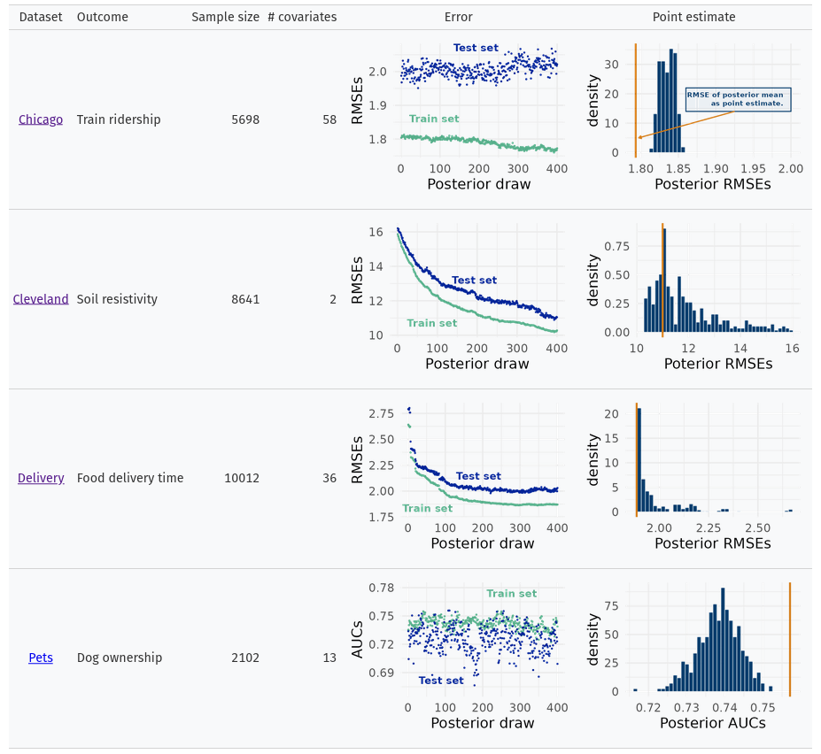
On 4 real datasets, see BART’s consistent performance over train/test splits.
On the right, the histogram indicates evaluation metrics for each posterior draw. The orange line is the evaluation metric of using the average across the posteriors as the BART point estimate.
A.3 Random effect BART
stochtree allows users to embed random effects alongside a BART term in a larger model. DESCRIBE. The data are from the agridat R package. Describe yields of barley at different Minnesota farming locations over different years as a function of weather conditions that year. Originally from (Immer and Henderson 1943), put together in (Wright 2013).
The data are natural for a random effect term because
With the data prepared, we now shift focus to modeling the data. The idea is to utilize Bayesian Additive Regression Trees (BART) (Chipman, George, and McCulloch 2012) with the stochtree software suite (Herren et al. 2025). Specifically, we use the stochtree implementation of XBART (He and Hahn 2023) to initialize promising BART forests.
As we have seen, BART is a carefully constructed model that is well equipped for prediction tasks. At its core, it represents an outcome \(y\mid \mathbf{x}\) through sum of regression trees (a “forest”). More formally:
\[
y = \underbrace{E(y\mid \mathbf{x})}_{\text{signal}}+\underbrace{\varepsilon}_{\text{noise}}=\underbrace{f(\mathbf{x})}_{\text{sum of trees}}+\varepsilon, \quad\varepsilon\sim N(0, \sigma^2)
\tag{A.1}\]
Each tree fits what the previous tree misses as in boosting. The trees are built probabilistically in a Bayesian way. There is a prior probability for growing a tree, which consists of choosing one of the \(\mathbf{x}_m, m=1, \ldots, p\) variables to split on uniformly at random, selecting a random position within the chosen \(\mathbf{x}_{m}\) that determines where the data is split by the tree1, and a prior distribution that gives a probability to stop growing a tree of a certain size. When the tree is built, which passes the outcomes \(y\) into buckets based on how the inputs \(\mathbf{x}\) were split up the tree, prior distributions are placed on the value that is drawn within the data in each tree bucket. Finally, a prior distribution is placed on the error term \(\sigma^2\). All the priors were constructed such that tree structures are relatively simple, the values drawn in the trees are relatively small, and the error term is relatively conservative. The idea is that prior to seeing data we assume \(f(\mathbf{x})\) can be constructed by summing together relatively simple trees that each contribute minimally to the overall fit of \(y\), so as to avoid over-fitting. But, if the data allow, the priors can be over-ridden and more complicated \(f(\mathbf{x})\) can learned.
1 so the data fall into left and right buckets depending on which side of the split rule they are categorized into.
The tl;dr is that BART can learn complicated relationships between inputs and how those impact the outcome/response \(y\). At the same time, BART predictions generalize well into the future and are reliable.
With stochtree, we modify Equation A.1 as follows:
\[
y = f(\mathbf{x})+\gamma_j+\varepsilon \longrightarrow y\sim N\left(f(\mathbf{x})+\gamma_j, \sigma^2\right)
\]
The modifications include placing a BART sum of trees model to have a random intercept \(\gamma_j\) for each farm location \(j=1, \ldots, K\), which is implemented in stochtree according to (Gelman et al. 2008). The random effect by farm location is included because of the natural grouping of replicates of each farm over the years that could be used to symbolize some sort of intrinsic features of the farm. On its own, having an input feature that can characterize difficult to measure intrinsic farm is valuable, and is a benefit of replicates. So simply including “site” as a column would likely help our model, at least from a predictive sense. Instead, we embed this information in a random intercept term for “site”. The random effects framework is preferable over just including a column indicator for multiple reasons. The random effect estimation process allows some degree of regularization via the pulling of group (“site) means towards one another. Additionally, the random intercept term is sampled, lending some”interpretability” to the variability of yield by town. Finally, observations by town now have errors that are correlated, so errors by town are correlated over time. This is a consequence of having a random intercept that is grouped by farm.
The final modification is to include an estimate of \(\hat{y}\) from a linear regression as a column into the \(\mathbf{x}\) covariate matrix. The thinking is that if there is a linear effect, trees can struggle to learn it without a lot of splits. This is a problem because BART is designed to avoid deep splits when tree building, so allocating too many splits to just the linear aspect of \(f(\mathbf{x})\) is troubling. If there is no linear effect, then there really is not a lot of harm with including one extra column into the regression. We also give this extra feature extra weight when splitting. This is coded as a user adjustable variable in this project. If we do not give extra probability to splitting on this feature and there are many features to split on, then including it is waste. If we put too much probability of splitting on just this column, then we can miss out on interactions and other aspects of \(f(\mathbf{x}))\) that are non-linear. In this example, since there are not many other features, we do not adjust the splitting probability.
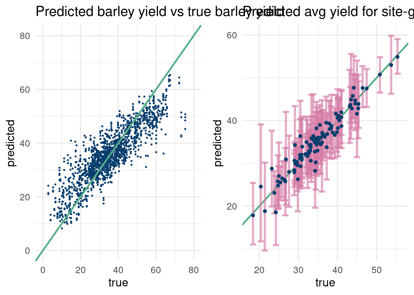
Train on 80% on of site-gen combos, test on 20% and averaging results per site-gen.
site_gen*
true
predicted
full_dist†
Crookston_Trebi
39.8
37.3
Duluth_Trebi
39.6
41.6
Crookston_WisconsinBarbless
39.3
36.6
GrandRapids_Peatland
29.7
30.3
Crookston_Colsess
31.0
33.9
GrandRapids_Odessa
24.7
25.8
Duluth_No474
33.1
34.3
GrandRapids_No474
26.5
26.1
* Actual yield.
† Intervals from 2.5 and 97.5% quantiles of full BART posterior, f(x) + random intercept & error uncertainty
Interactive mode.
The following code to replicate Figure A.1. We do not run this code as getting the aesthetics right requires manual editing based on the specific train/test splits. We don’t mess with the aesthetic.
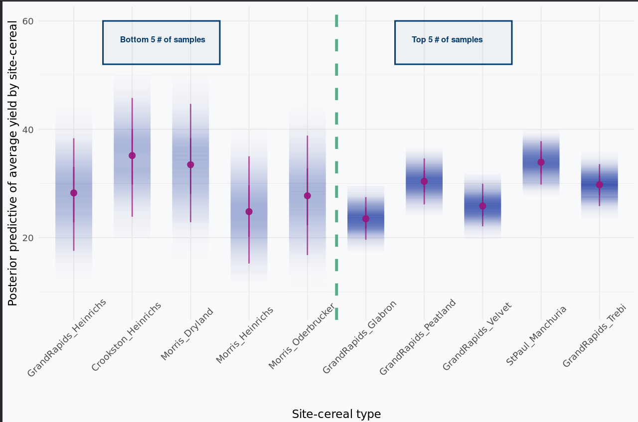
Look at full predictive posterior distributions for different number of replicates. Not run.
Figure A.1: The posterior distributions get narrower as the number of replicates increases, as expected. Uncertainty isn’t merely due to limited data (see aleatoric vs epistemic uncertainty).
A.4 Constraints
A.4.1 Great lakes and heteroskedastic noise
The data are from the National Oceanic and Atmospheric Administration (noaa) government site and describe the surface temperature on Lake Superior year over year. Specifically, the following link will bring you directly to the .txt file on noaa’s site. Also have data for the other lakes, and it’s pretty easy to download historical data for any of the great lakes. We zone in Fahrenheit because the granularity is nice.
The first modification to the base BART model is to take the log of the outcome, which has the benefit of ensuring positive predicted surface temperatures and also imposes the assumption of a log-normal distribution of surface temperatures, which is more realistic than normally distributed surface temperatures according to exploratory data visualizations. Incorporating hard constraints into BART is tricky, as we need to grow the trees (and subsequently the forest) with the constraints in mind. This would require accounting for the constraint when trees are accepted/rejected, which means modifying the marginal likelihood calculations. Rejecting forests that fail to meet the criterion post hoc violated the dependent structure of the MCMC, meaning you are not sampling from the stationary distribution (aka the posterior distribution).
So, in order to ensure the outcome is positive (including the posterior predictive intervals) we actually model: \(\log(y) =f(\mathbf{x})+\varepsilon\), which means that \(y\) is log-normally distributed:\(y\sim\exp[N\left(f(\mathbf{x}),\sigma^2(\mathbf{x})\right)]\). This also means the \(\sigma^2(\mathbf{x})\) now represents a multiplicative error and is interpreted on a scale of the percentage of \([f(\mathbf{x})]\). This is because \(y=\exp(f(\mathbf{x})+\varepsilon)=\exp(f(\mathbf{x})\exp(\varepsilon))\), which means the mean forest, the random intercept and error terms are now interpreted as “multiplicative” of one another, were we to try and analyze each term on its own. So a value of 1.01 on this scale means we multiply the other terms in the model by 1.01, i.e. a 1% increase.
You might wonder why not use a log-linear BART prior to model this outcome. This is certainly possible, but is a little overkill. Heteroskedastic BART in stochtree uses the log-linear BART prior from (Murray 2021) since only \(\sigma(\mathbf{x})\) has to be positive, but \(f(\mathbf{x})\) and \(y\) do not need to be. In our case, only \(y\) has to be positive, which makes life easier.
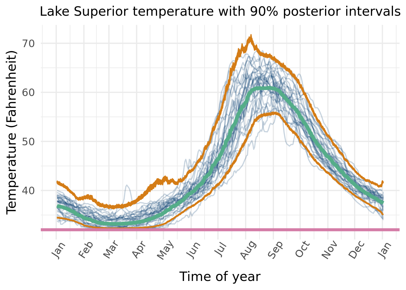
Speaking of heteroskedastic forests, we also include a “heteroskedastic forest” to learn \(\sigma(\mathbf{x})\). The heteroskedastic forests give allow the variance term in the error to be learned from the data. Looking at the temperature data over the course of the year, there is a lot more deviance from the average in the summer compared to the other seasons.
Code to run a heteroskedastic BART regression.
options(warn=-1)suppressMessages(library(stochtree))suppressMessages(library(tidyr))suppressMessages(library(tidyverse))# Source:# https://coastwatch.glerl.noaa.gov/statistics/average-surface-water-temperature-glsea/df_init =read.csv(paste0(here::here(),'/data/Superior_all_year_glsea_avg_s_F.csv'))df =read.csv(paste0(here::here(),'/data/Superior_all_year_glsea_avg_s_F.csv'))df$day = df$Xdf = df %>% dplyr::select(-X)df = df %>%pivot_longer(cols =starts_with("X"), # Selects columns that start with "Test"names_to ="Year", # Name for the new column holding the original column names (e.g., "Test1")values_to ="Temp"# Name for the new column holding the values (e.g., 85, 92) )num_gfr <-25num_burnin <-10num_mcmc <-200num_samples <- num_gfr + num_burnin + num_mcmcgeneral_params <-list(sample_sigma2_global = F, verbose=F, num_chains=20)mean_forest_params <-list(num_trees =25,alpha =0.95, beta =2, min_samples_leaf =5)variance_forest_params <-list(num_trees =5, alpha =0.95,beta =3, min_samples_leaf =30)df = df %>%drop_na()fit = stochtree::bart(X_train =as.matrix(as.numeric(df$day)),y_train =log(as.numeric(df$Temp)-32),num_gfr = num_gfr,num_burnin = num_burnin,num_mcmc = num_mcmc,mean_forest_params = mean_forest_params,general_params = general_params,variance_forest_params = variance_forest_params)yhats2 <-exp(fit$y_hat_train[, ] +sqrt(fit$sigma2_x_hat_train[,])*rnorm(length(df$day)*(fit$model_params$num_samples)))yhats <-matrix(rlnorm(length(df$day)*(fit$model_params$num_samples), fit$y_hat_train, sqrt(fit$sigma2_x_hat_train)), ncol=ncol(fit$y_hat_train),nrow =nrow(fit$y_hat_train))qm =apply(yhats2,1, quantile,probs=c(.05,.95))df2 =data.frame(X =as.numeric(df$day),y =as.numeric(df$Temp),bart =exp(rowMeans(fit$y_hat_train)),LI = qm[1,],UI = qm[2,])df2$X =as.Date(df2$X, format ="%j", origin ="1.1.2014")index =unlist(lapply(1:length(unique(df2$X)),function(k)seq(from=1,to=sum(df2$X==unique(df2$X)[k]))))df2$index = indexplot2 <-ggplot(df2, aes(x=X, y=y, group=index)) +geom_line(color='#073d6d', size=0.67, alpha=0.22)+scale_x_date(date_breaks ="1 month", date_labels ="%b") +geom_line(aes(x=X,y=bart+32), color='#55AD89', lwd=2, lty=1)+geom_line(aes(x=X, y=LI+32), color='#d47c17', lwd=0.72,alpha=0.95, lty=1)+geom_line(aes(x=X, y=UI+32), color='#d47c17', lwd=0.72,alpha=0.95,lty=1)+geom_hline(aes(yintercept=32), col='#d47ca7', lwd=1.75)+ylab('Temperature (Fahrenheit)')+xlab('Time of year')+ggtitle('Lake Superior temperature with 90% posterior intervals')+theme_minimal(base_family ="Roboto Condensed", base_size =16)+theme(#axis.text.y = element_blank(),#axis.ticks = element_blank(),axis.text.x =element_text(angle =57, hjust =0.63),# strip.text.y = element_blank(),plot.background =element_rect(fill='#ffffff', #e6f1f7',color=NA),plot.title=element_text(hjust=0.5, size=16))plot2
Without the log-transformation, we could get temperatures below 32 (Fahrenheit) for the predictions, but we know this violates physical law that water cannot be liquid below 32. So the Lake’s minimum temperature is 32 degrees, when it is all ice.
A.4.2 Hacky prior predictive
In the previous section, we discussed the log-transform to incorporate the constraint of positive outcomes. Another (again hacky) way to do this is to use the kernel representation of BART and then incorporate the constraint through rejection sampling. (Geweke 1991). Since the multivariate normal can be sampled without using MCMC methods, we do not need to worry about rejecting samples post-hoc. It is not extremely efficient, as say we have 100 points. That is a 100-dimensional multivariate normal! Based on what our bounds are, we would have to reject the entire sample if just a single point of the 100 from a generated multivariate normal falls outside the bounds. This means we might need to sample MANY times to get a sufficiently large sample from the multivariate distribution2.
2 We will show this with a print statement in the code.
There is a catch with this approach. It isn’t BART anymore. It is starting with the implied distribution from the BART forests, but the constraints reject samples that would be valid BART samples. The BART forest construction, so heralded for its accuracy, has no input into the forests we sample using the rejection method on the multivariate normal kernel BART representation. In other words, the functions we sample using this method are decidedly not BART with a constraint, but they obey the constraint using BART as a building block. REWRITE THIS CONFUSING PARAGRAPH.
Chipman, Hugh A and, Edward I George, and Robert E McCulloch. 2012. “BART: Bayesian Additive Regression Trees.”Annals of Applied Statistics 6 (1): 266–98.
Gelman, Andrew, David A Van Dyk, Zaiying Huang, and John W Boscardin. 2008. “Using Redundant Parameterizations to Fit Hierarchical Models.”Journal of Computational and Graphical Statistics 17 (1): 95–122.
Geweke, John. 1991. “Efficient Simulation from the Multivariate Normal and Student-t Distributions Subject to Linear Constraints and the Evaluation of Constraint Probabilities.” In Computing Science and Statistics: Proceedings of the 23rd Symposium on the Interface, 571:578. Fairfax, Virginia: Interface Foundation of North America, Inc.
He, Jingyu, and P Richard Hahn. 2023. “Stochastic Tree Ensembles for Regularized Nonlinear Regression.”Journal of the American Statistical Association 118 (541): 551–70.
Herren, Drew, Richard Hahn, Jared Murray, Carlos Carvalho, and Jingyu He. 2025. Stochtree: Stochastic Tree Ensembles (XBART and BART) for Supervised Learning and Causal Inference. https://stochtree.ai/.
Immer, FR, and MT Henderson. 1943. “Linkage Studies in Barley.”Genetics 28 (5): 419.
Murray, Jared S. 2021. “Log-Linear Bayesian Additive Regression Trees for Multinomial Logistic and Count Regression Models.”Journal of the American Statistical Association 116 (534): 756–69.