We generally prefer a Bayesian approach, and will soon tell you why in a curated list. We will caveat a few things first though:
There are many concepts in statistics that are neither Bayesian or frequentist. Likelihoods are important in both, for example. Frequentist coverage can be evaluated in simulation studies with Bayesian estimators. Similarly, evaluation metrics for Bayesian methods can also be calculated for frequentist estimation approaches.
Use the method that makes sense for the problem at hand. You do not have to shoehorn a Bayesian (or frequentist) method because it is what you know and you want to be a zealot.
Bayesianism doesn’t solve all your problems. If a quantity can’t be estimated from infinite data (i.e. its unidentifiable), then no prior will help you. If the data present little to no signal, again the prior can only do so much. If the goal is to predict an outcome, it certainly won’t help. (Gelman and Shalizi 2013), paper here, argue that estimating a posterior, which is then used as a prior for future studies, does not end an analysis. Rather, a model should still be held to intense scrutiny, and you may need to re-calibrate your Bayesian model, or start completely anew. The authors argue this deductive workflow is a strength of Bayesian statistics, as it is easy to validate your model and check for wonkiness.
The power of Bayesian inference here is deductive: given the data and some model assumptions, it allows us to make lots of inferences, many of which can be checked and potentially falsified. For example, look at New York state (in the bottom row of Figure 3): apparently, voters in the second income category supported John McCain much more than did voters in neighbouring income groups in that state. This pattern is theoretically possible but it arouses suspicion. A careful look at the graph reveals that this is a pattern in the raw data which was moderated but not entirely smoothed away by our model. The natural next step would be to examine data from other surveys. We may have exhausted what we can learn from this particular data set, and Bayesian inference was a key tool in allowing us to do so.
Their Bayesian model turned out to not be particularly useful, despite having well designed prior specifications and working well 4 years earlier. To a data scientist, this cycle of something working until it doesn’t and constantly checking that its still kosher is not new. In fact, the data scientist would be proud of the statistician who admits their model took a beating and maybe needs to be retired.
Anyways, we promised a list of arguments for the Bayesian school of thought and we are nothing if not honest. The following \(8\) points are not wildly different than those championed (tepidly endorsed?) by Andrew Gelman here1.
1 In fact, the decision analysis bullet point was omitted in a previous version of these notes, so credit to the Statistical modeling blog and Andrew Gelman for emphasizing this important topic. While discussed in greater detail in later chapters, with an emphasis on its importance, curiously the decision analytic viewpoint was forgotten. Ain’t that just the way.
Sensible probablistic viewpoint (adheres to likelihood principle): It is seemingly a more coherent view of probability, more natural for most people than the frequentist approach, which typically says a parameter is fixed. To get around this, however, a prior distribution over what the researcher thinks the model should be and where its mass should lie must be introduced (in addition to specifying a model of the likelihood). Bayes offers an arguably more proper interpretation of probability, at least for many practical problems of interest. In contrast, p-values violate the likelihood principle (imagine flipping a coin 10 times and seeing how many times you get exactly 2 heads or think about flipping a coin 10 times until you get two heads —> same likelihood, different p-values , true p-value and confidence interval interpretation. Additionally, a Bayesian treats their observed data as what we condition on2. The underlying parameter that generated that data comes from a probability distribution. Their is a prior distribution for the parameters and a distribution that we learn given the observed data. The frequentist approach fixes the underlying (unobserved) parameter, but imagines if the data had been collected hypothetically so many times, this is what you would expect to see…except we only ever do see one outcome. This leads to a lot of confusion about confidence intervals, with most people’s interpretation of “the probability the truth is in this range” actually belonging to the Bayesian paradigm due to the application of Bayes theorem yielding the probability of interest. In other words, we get a probability for the “model” (the parameters in the model) given observed data, meaning we average over possible values of the parameter and the observed data! However, this comes at the expense of specification of a prior distribution for the parameter(s), which could be wrong! So it goes.
The prior is your friend (prior information and/or regularization mechanism): The idea of a prior allowing a researcher to incorporate more information and potential constraints in a principled way. This can be particularly useful when we do not have a lot of data but have a good feel for what our future data may hold. For example, in hierarchical modeling, the famous introductory example is actually from baseball! If a player does not have a ton of bats, yet has a high batting average, what should we expect of this player? Should we entirely discount their hot start and just assume they go back to an average player? Or should we ignore the rest of the league and buy into the small sample tea leaves? A hierarchical model allows us to sort of weigh these two options, through a statistical phenomenon called shrinkage. Basically, a-priori we assume some of the hot start is an aberation which has the effect of pulling the player’s true performant ability closer (but not entirely) to the league average. Further information can be encoded into the model through priors. Prior values can be chosen to reflect how these scenarios for batting average played out in years past or for other players identified as similar in past years (similar defined by another statistical model or the “eye”). Beta-Binomial is another good starting example of information being encoded into a problem through the prior, which we discuss soon.
Prior predictive distributions allow us to look at probability distributions of expected data averages over the values of the chosen prior distributions in a model, which is a really wise thing to do.
Predictive capabilities: Bayesian methods are a little more natural in terms of a predictive sense (posterior predictive). You can model very complicated things with simpler models (think the Gibbs Sampler). Bayesian methods also allow us to more easily overcome difficult problems in traditional statistics, such as small sample sizes in a regression model, or a regression with a large amount of variables. Additionally, as we will see in chapters 8 and 9, designing regularization priors can be extremely helpful for improving predictive capabilities and trust-worthiness of a modeling regime.
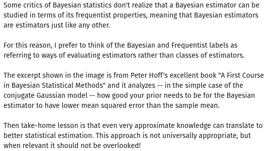
3a) Nice sampling properties: Additionally, sometimes Bayes estimators actually have better (frequentist) statistical properties. Chapter 5 of (Hoff 2009) shows an example of this, where for a given value of a parameter (the point estimate), one can show when the Bayes estimator of the mean of a normal distribution has a lower mean squared error of the truth than the frequentist estimate (which is the sample mean of the observed variance via a maximum likelihood calculation). The comparison depends on the priors on the mean and variance parameter you choose, but there are certain priors that show that the Bayes estimator is “better” (via MSE as a metric).3 The idea that Bayesian estimators can have better sampling properties adds an extra (but very similar) flavor besides just incorporating more information into our models or introducing an intentional bias to avoid over-fitting.
De Finetti: De Finetti’s theorem provides justification in terms of Latent Variables. if observables are exchangeable4, then there exists an underlying latent θ that generates the data. This is nice because De Finetti says that if the observable things are exchangeable, then there exists an underlying parameter. In other words, if permutations of random variables are the same, then this theorem implies there is a root/common factor that generates those data, thus giving some theoretical backing to Bayesian statistics! Perhaps more interestingly is the role of De Finetti’s theorem in the predictive sense. Because De Finetti relates observable variables to an unobserved generating variable, it is natural then to think of predictive distributions (prior or posterior), where we study what observations are expected to look like given the prior distribution of the parameter (or the updated posterior distribution of the parameter). Future observations are an average of the likelihood of observed data, with the weights in the average determined by the distribution of the generating parameter. This can be done prior to seeing data (prior predictive, which generates hypothetical data that could be observed) or after observing some data and updating the parameter(posterior predictive).
Bayes Rules: are admissible (eh)…they are not always worse for sure!
Marginalization vs optimization: If we have a model parameter (say we have a linear model \(y=mx+b\), we generally would try and find the parameters would be the \(m\) and the \(b\) which informally make the line “look” the best) , frequentist methods usually want to find the “best” value of this fixed quantity. Bayesian methods marginalize, or ignore, this parameter by taking a weighted sum of the data with the weights determined by the prior distribution of the parameter, i.e. weighted by more likely outcomes. This is the “normalizing constant” that makes Bayesian statistics hard, but could be more useful computationally. Another way to think of this is a Bayesian perspective typically incorporates a stochastic search over the model space versus a gradient descent that is going in the most optimal ways to search for the best parameter.
A natural way to quantify uncertainty: This arises because posterior distributions are actual probability distributions in a very natural sense. We can study the distribution of parameters after seeing data (made possible by specifying a prior distribution for these parameters). We can also see an entire distribution of predicted values of our data given “training data” (posterior predictive distributions). In chapter 8, we consider priors priors over function space, which are pretty cool and arguably more intuitive. Bayesian non-parametrics! Uncertainty quantification of estimated functions seems even more important.
Bayes risk & decision analysis: Bayesian analysis is often found accompanying decision analysis. With a utility function (which is the negative of a loss function, such as mean squared error), we can calculate the risk of an estimator (the average loss of an estimator) with respect to prior. Following the exposition in (Casella and Berger 2002): \[\text{Bayes risk} = \int R(\theta, \hat{\theta})\pi(\theta)\text{d}\theta=\int_{\Theta}\underbrace{\int_{\mathcal{X}} \mathcal{L}(\theta, \hat{\theta})f(\mathbf{x}\mid\theta)\text{d}\mathbf{x}}_{\text{average loss}}\pi(\theta)\text{d}\theta \tag{3.1}\]
Where \(\mathcal{L}\) depicts a loss function, \(f(\mathbf{x}\mid \theta)\) is the likelihood function of the data generated by a parameter \(\theta\), and \(\pi(\theta)\) is the prior probability distribution of the parameter. The average loss is the average deviation5 of an estimator \(\hat{\theta}\) from \(\theta\), i.e. the average value of the loss function averaged over the observed data. This value is then averaged again, with the “weights” determined by the prior distribution of the parameters (since an average is a weighted sum, and the integral is a generalization of the summation). We can re-arrange Equation 3.16 and see that the Bayes risk is actually the posterior expected loss. Given an entire posterior distribution, a natural question is how to choose an estimator to describe as the “best” one. With respect to our prior choices (on the parameters that generate the data) and the data, which estimator is the best on average. Should we use the mean? The median? The mode? Bayes world provides a nice way to think about this problem, considering both the data and the parameters and calculating the expected loss of the posterior distribution of the parameters.
The main benefit to the Bayesian mode of thinking for decision analysis is that the risk integral is taking with respect to the prior distribution of the parameters, which is in contrast with the frequentist definition of risk. Rather than considering different data than what we observe, The Bayesian assumes the data is indeed known. The frequentist would fix the generating parameters, \(\theta \in \Theta\), and instead average the loss over unseen but hypothetical new values of the data \(\mathcal{X}\) generated by a fixed \(\theta\). See this nice stackoverflow link for a discussion of the benefits of a Bayesian approach over the frequentist alternative.
2 Confusingly, the observed data are still generated from a random variable…the likelihood is still a crucial part of Bayesian methods after all.
3 Of course, they also could be a lot worse!
4 Exchangeable refers to the notion that the ordering of the observed data does not matter. For example, tomorrow and todays data come from the same distribution.
5 Where deviation could be the squared distance (\(\theta-\hat{\theta})^2\), the absolute value, or other distance functions quantifying the dis-similarity of \(\theta\) to \(\hat{\theta}\).
6 By using Bayes rule to see that: \(f(\mathbf{x}\mid \theta)\pi(\theta)=\frac{\pi(\theta\mid \mathbf{x})}{\int f(\mathbf{x}\mid \theta)\pi(\theta)\text{d}\theta}\)
3.1 On the role of the prior
Loosely, the likelihood in statistical modeling stipulates your data (such as an outcome \(y\)) can be described by distribution(signal, noise). The signal is estimated by a model (function really) with parameters, and the noise is also modeled by a parameter (or function of parameters if you wanna be fancy). Any parameter is a random variable and therefore needs a prior distribution on where we expect the value of the parameter to reside.
The prior is an interesting, and widely discussed aspect of Bayesian statistics. Broadly speaking, the prior refers to the distributions of the parameters in your model set before seeing any data7. To some, it is a way to incorporate additional information into a problem. To others, it can be used to constrain the search space. …
7 although it can be informed from previous experiments
In “frequentist” statistics (the idea that statistics is based off hypothetical repeated sampling) parameters are considered fixed and unknown values. Data (\(X_1, \ldots, X_n\)) are drawn according the parameter (\(\theta\) ). Typical approaches include finding the \(\theta\) that make the observed data as likely as possible. This framework assumes that \(\theta\) is a fixed value, meaning the probability of observing it is a 1 or 0, and concepts of statistical inference are built off hypothetical repeated samples of the observed data (which we only observe once…). This sort of counter-intuitive framework, to me at least, helps explain why the definitions of p-values and confidence intervals are so confusing to people learning, and practicing, statistics. Can’t we just have an interval where we can say “there is a 95% probability of the mean lying in this range”? Yes!
IDK one of those check the conditioning fun examples
3.3 Back to Bayesian statistics
From Bayes rule, if we transition from events \(A\) and \(B\) to sampling models of data \(\mathbf{x}\) associated with generating parameters \(\theta\), we will begin the transition to traditional Bayesian statistics as it is implemented in practice.
Using Bayes rule, described above in Equation 3.2, we can actually relate a likelihood \(L(\mathbf{x}\mid \theta)\), a prior, \(\pi(\theta)\), and a posterior \(\pi(\theta\mid \mathbf{x})\). The likelihood is our sampling distribution, aka a “data generating process (DGP)” and can loosely be thought of as the model of the data. The prior is the distribution of the parameters that generate the likelihood, which we have to specify before seeing data. The relation is then given through Bayes theorem:
The numerator in Equation 3.3 is the likelihood times the prior. The denominator integrates the numerator by all the possible values of the prior, which normalizes the distribution to 1. It is also called the “marginal likelihood”, since we marginalize/ignore the effect of \(\theta\)8. The marginal likelihood can be understood as the probability of the data (given a prior for the associated parameters of the model). The left hand side of the equation, \(\pi(\theta\mid\mathbf{x})\), is a valid probability distribution of the parameters in a model conditional on the observed data.
8 The term “marginalizing” comes from summing the rows of a column and putting this sum in the margins, thus marginalizing the effect of the variables that are “discarded”. Intuitively, the marginal probability of X is computed by examining the conditional probability of X given a particular value of \(\theta\) and then averaging this conditional probability over the distribution of all values of \(\theta\). So we are looking at the average (with respect to the prior distribution on \(\theta\)) value of the likelihood for the observed data.
A way to think about this term is that since marginalizing incorporates all values of the prior, then the process essentially is a guided search of the likelihood over the more probable regions of the parameters as dictated by the prior choice. In this sense, it refers to the probability of observing the sample of data we did over all values of the prior, which is why it is sometimes called the “model evidence”. (McElreath 2018) calls is the “average likelihood”, as it represents the average value of the likelihood over all the possible values of the specified prior. Remember, an average is a weighted sum (or integral in the limit) of the random variable you want to find the average of. In our case, the likelihood function is weighted by the prior distribution on the parameters, which gives weights to how probable values parameter values being multiplied by the likelihood are. In effect, low probability parameter scenarios (as dictated by chosen prior) contribute to the average likelihood less, by mutliplication with of the likelihood of a smaller number. Of course, the likelihood can still “over-ride” this, as the prior serves more as a “guide” then a steadfast rule. This is a nice feature of the Bayesian framework. Chapter 5 of (Williams and Rasmussen 2006) gives a really nice description of the marginal likelihood, in particular figure 5.6 of the 2006 version, which can be found here.
Specifically, (Williams and Rasmussen 2006) describes the “average likelihood” (okay marginal) through the lens of Occam’s Razor. To summarize the description in our own words, imagine we have three worlds of data generating processes. We see a world where the outcomes (\(y\) ’s) are generated from a linear process, a sinusoidal (periodic) process, or a polynomial (say quadratic or cubic) process. These are the only three types of data we could ever see. We have two models available to us (for which all the parameters in said models constitute a prior) to “fit” these data. One is a simple linear model, and the other is a complicated machine learning model (say a Gaussian process with a squared exponential kernel or a neural network). The marginal likelihood summed (well integrated) over all possible data generating processes is a valid probability distribution (over the possible range of outcomes \(y\)) and thus must sum to 1. In fact, this is called the prior predictive distribution. So the prior predictive distribution evaluated at data generated from the “linear world” will yield a high marginal likelihood. This is since prior predictive distribution for these particular data has the interpretation of the likelihood of the data averaged over the values of the prior9. Conversely, a linear prior will yield a low marginal likelihood for the sinusoidal or polynomial data, because non-linear data is unlikely to have been generated from a linear model. The complicated model will be well equipped to fit any of the three data “worlds”. Since the prior predictive distribution over all the data generating “worlds” must sum to one, the complicated model will have nearly equivalent marginal likelihoods for each of the worlds. So if we were to compare the prior predictive distribitions as a way to select a model to fit our data, the linear model would be preferred over the complicated one in the case of a linear data generating process, even if they fit the data with equal accuracy!
9 Where the prior parameters could the possible combinations of slopes and intercepts in the linear model or the weights on neurons in a neural network.
Frequentist techniques do not treat the parameter as a random variable, which means this approach cannot be used there; instead a value of the parameter is chosen and the likelihood is evaluated; the parameter is chosen typically to make the likelihood as “likely” (large) as possible, a technique called “maximum likelihood estimation”. The Bayesian too use maximum likelihood, though typically maximize the marginal likelihood, a technique called “type II maximum likelihood” or “Empirical Bayes”.
The marginal likelihood is also strongly related to a concept called the prior predictive, which will discuss in the Simulations mini-chapter. For a prior predictive, we specify a likelihood and take the average with respect the prior to see what outcomes the prior would predict (of course prior to seeing any actual observations), which is what the integral in the marginal likelihood is doing. The difference is that the prior predictive distribution does not account for observed data, but rather can be thought of as simulating from potential data in the support of the likelihood function, weighted by our choice of prior10. So the chosen distribution on the prior for the parameter(s) is consequential and this is one to see what types of data we might expect to see were the world generated by the prior we prescribe.
“More importantly for our considerations here, if we do not evaluate the marginal likelihood at our data then it becomes a predictive distribution for the data supported by the prior or the prior predictive distribution.”
The following code, a modification of a homework from Dr. Hedibert Lopes class, illustrates one way one could calculate a posterior. Of course, the difficulty lies in the integration of the marginal likelihood. Without it, we do not have a valid probability and just have numbers for a posterior, and we have no way to know how to scale that number properly without doing the integral. Generally, save for conjugate prior analyses (which we will soon talk about), the integral cannot be analytically solved, and a number of computational tools, such as Markov Chain Monte Carlo methods, Gibbs samplers, and the Metropolis Hastings algorithm (all of which are related to one another as we will soon see) have been developed to approximate the integral. However, since this problem is one dimensional, we will brute force a solution to the integral by evaluating a fine grid of rectangles and sum them up, which is how integration is taught after all. We do so on a grid of 1000 points (which may not even be enough), which should show why this method won’t scale: in 3 dimensions we would need 1 billion evaluations, which is already pushing our computer, and a 3 dimensional model is not very large in common statistical practice.
We want to study the Binomial model, which is a generalization of the Bernoulli model (the coin-flip model). Specifically, we want to model the number of successes, \(s_n=\sum_{i=1}^{n}x_i\), which yields a likelihood
\[
L(\theta\mid n, s_n)=\frac{n!}{s_n!(n-s_n)!} \theta^{S_n}(1-\theta)^{n-s_n}
\]
Assume a Beta(a,b) prior. The posterior can be derived analytically:
where we skipped a few steps. In the code below, we will calculate the marginal likelihood, the normalizing constant, through numeric integration and ignore all the lengthy calculations we did above :( to basically prove a point.
Click here for full code
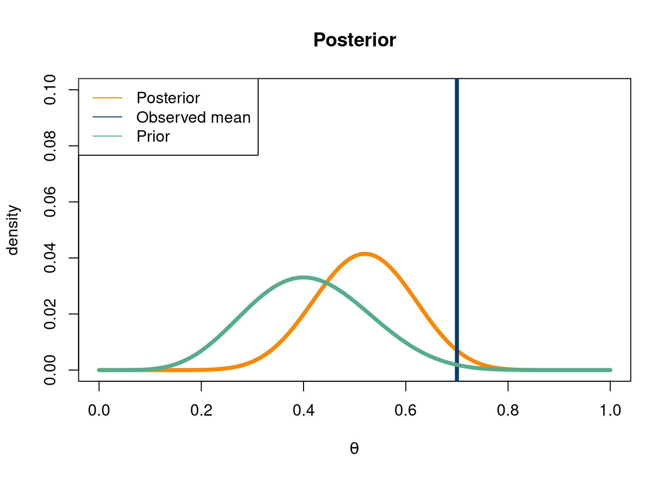
# Calculate the marginal likelihood.grid <-seq(from=0, to=1, by =0.01)N <-1/0.01mu <-0sigma <-3theta = grida =7b =10n=10sn=7integrate_function=function(theta,a,b){n=10sn=7likelihood_term1 <-factorial(n)/(factorial(sn)*factorial(n-sn))likelihood_term2 <- theta^(sn)*(1-theta)^(n-sn)likelihood <- likelihood_term1*likelihood_term2prior =dbeta(theta,a,b)#alternatively, an easier approach using built in R functionslikelihood <-dbinom(sn, size=n, prob=theta)return(sum(prior*likelihood,na.rm=T)/length(theta))}# divide by grid size to do Riemman integralnorm_constant <- N*integrate_function(grid,a,b)prior=function(theta,a,b){return(dbeta(theta,a,b))}likelihood =function(theta,sn,n){return(dbinom(sn, size=n, prob=theta))}theta =seq(0,1, by=0.01)#### PLOT PRIOR and Posterior #####define rangetheta =seq(0,1, by =1/N)#### Prior C ####plot(theta,(likelihood(theta,sn,n)*prior(theta,a,b))/norm_constant,xlab=expression(theta), ylab='density', type ='l', col='#FD8700',main='Posterior', lwd=4, ylim=c(0,0.10))abline(v=sn/n , col='#073d6d', lwd=4)lines(theta, prior(theta,a,b)/N, col='#55AD89', lwd=4)#add legendlegend('topleft', c( 'Posterior', 'Observed mean','Prior'),lty=c(1,1),col=c('#FD8700','#073d6d', '#55AD89'))
Click here for full code
#should sum to 1sum(likelihood(theta,a,b)*prior(theta,a,b))/norm_constant
[1] 1.01
Click here for full code
#plot(integrate_function(grid,1,7), xlim=c(1,31))
So, basically \(1\), as expected. You could also use the integrate function in R to calculate the value of the denominator, which again is feasible in this one-D example. The answers will differ slightly because our grid was not super tight in the “by-hand” calculation.
Expand to see code to compare integrate function and by-hand
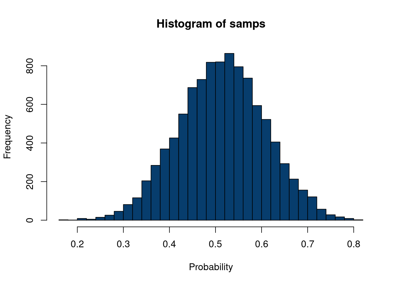
How do we sample this way? Well, with the normalizing constant in hand, we have a list of probabilities, meaning we can take advantage of the “sample” function in R to great use.
Click here for full code
integrate_function=function(theta,a,b){n=10sn=7likelihood_term1 <-factorial(n)/(factorial(sn)*factorial(n-sn))likelihood_term2 <- theta^(sn)*(1-theta)^(n-sn)likelihood <- likelihood_term1*likelihood_term2prior =dbeta(theta,a,b)#alternatively, an easier approach using built in R functionslikelihood <-dbinom(sn, size=n, prob=theta)return(prior*likelihood/length(theta))}# divide by grid size to do Riemman integralpost_weights <- N*integrate_function(grid,a,b)samps =sapply(1:10000, function(k)sample(theta, size=1, prob=post_weights))hist(samps, 30,col='#073d6d', xlab='Probability')
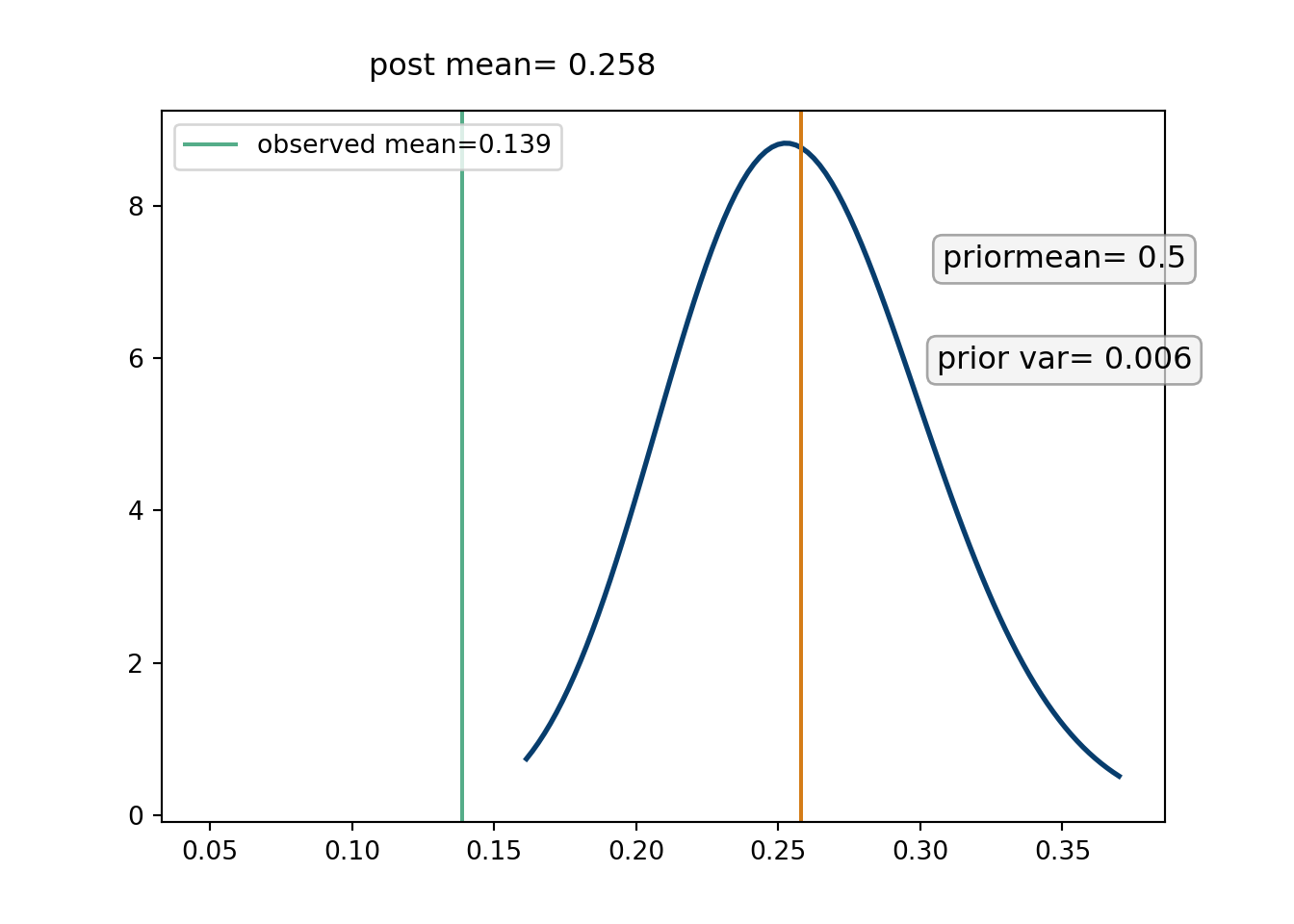
Alright, lets get back to our applied example. We want to look at the impact of the \(a\) and \(b\) parameters of the prior. In his career, as of the end of the 2023-2024 NBA season, Ben Simmons is \(5/36\) on 3-pt shots (which is about \(13.9\%\)). This is shockingly little data, so we put a prior on the proportion of shots we expect Simmons to hit in 2024/2025. We could do an “informed” prior by setting \(a\) and \(b\) to be what we would expect a high level point guard’s 3pt data to look over a season (for example Jalen Brunson made \(211/526\approx 40.1\%\), but that is very heavy handed prior guidance. Instead, we will just try some different values and see what it does.
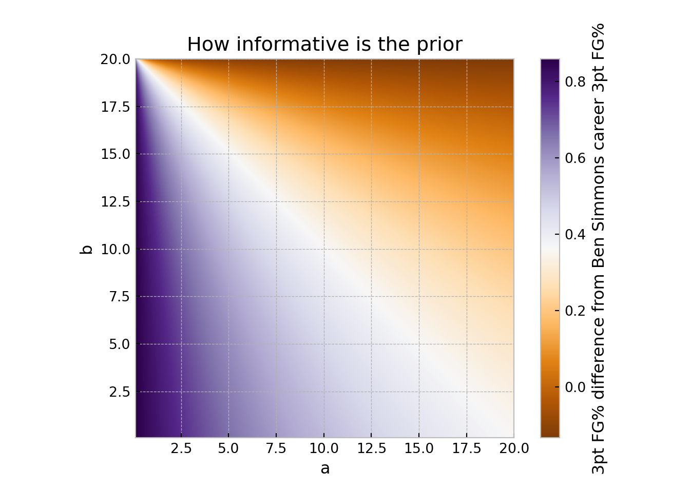
Now, let’s look at varying the prior parameters through a grid approach.
Click here for full code
# Distance implied by a and b parameters# How far away do these priors make us from Simmons career# Calculate the posterior means and compare to prior meansdef dist(apr,bpr): mean=apr/(apr+bpr) var=(apr*bpr)/((apr+bpr)**2*(apr+bpr+1))return(mean-p)#np.sqrt((mean-p)**2+(var-simvar)**2))#grid search method!distlist=[]distlistalt=[]N=500amin=0.1amax=20bmin=0.05bmax=20alist=np.linspace(amin,amax, N)blist=np.linspace(bmin, bmax, N)for i in alist:for j in blist: distlist.append(dist(i,j))#plt.imshow(np.array(distlist).reshape(500,500))mpl.style.use('bmh')distarr=np.array(distlist)distreshape=distarr.reshape(N,N)fig,(ax) = plt.subplots(1,1, figsize=(7,5))im=ax.imshow(distreshape,extent=[amin, amax, bmin, bmax], cmap='PuOr')plt.xlabel('a')plt.ylabel('b')fig.colorbar(im, orientation='vertical', label='3pt FG% difference from Ben Simmons career 3pt FG%')
<matplotlib.colorbar.Colorbar object at 0x7a33c2bee9e0>
Click here for full code
plt.title('How informative is the prior')plt.show()
The role of the prior is one that many statisticians have argued about for years. A Bayesian skeptic argues that one can choose their prior to have a strong influence over their posterior given they do not trust their data. On the other end of that spectrum is to pick very agnostic priors, such as a uniform prior, which express the belief that the parameters value is relatively unknown to the researcher a priori. A third approach is to try many different priors as a sort of sensitivity analysis.
Our view of the prior is that it can serve as a sort of “guide” in the search of a parameters posterior distribution. Encoded in the prior are beliefs over where the parameter lies and where it is most likely. In the integration stage, the prior then guides the posterior search, which itself describes the probability of the models parameters given the observed data. A prior can serve as a regularizing agent, encouraging simpler models. The prior can encode a constraint that we know a physical system should have. In a Gaussian process framework (more on that later), the prior (specified by the so-called “kernel”) dictates which functions we can sample from, which even after seeing data, affects the shape of the predicted function. In a BART (Bayesian additive regression tree) prior11, trees are strongly influenced by the tree growing prior, which encourages small trees (in the absence of data). Of course, the data (through the likelihood function) plays a huge role in the shape and scales of the posterior distribution, and this next example should help illustrate that.
11 Which we will be well acquainted with by the end of these notes
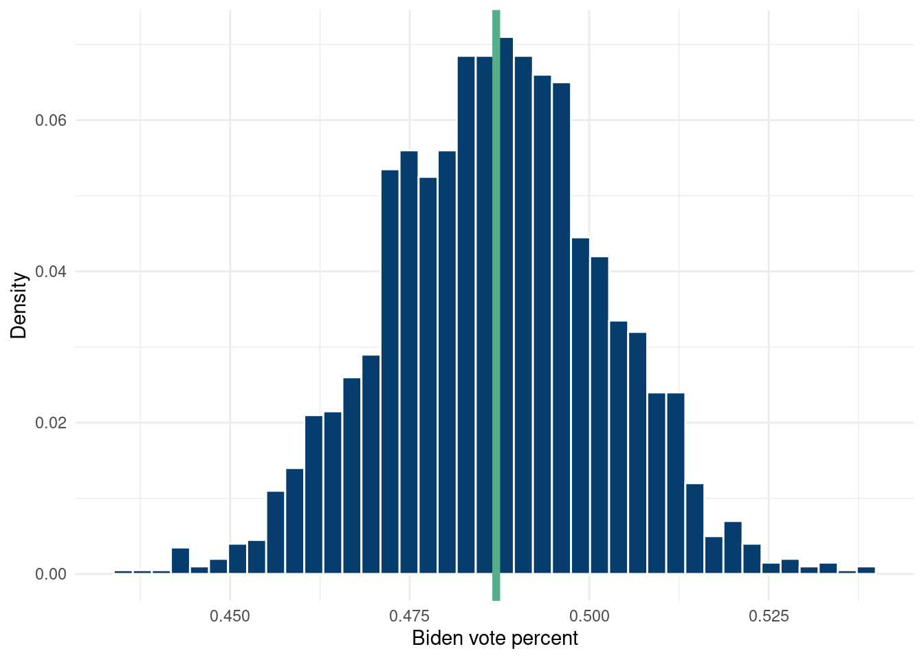
3.4 The beta bernoulli for election polls
This type of conjugate prior analysis is nice because one need only access the awesome conjugate prior wikipedia page to proceed with their analysis. Here is a Cool tutorial. We are kind of belaboring the beta-Bernoulli at this point, but we could do a similar analysis with other conjugate analyses.
Click here for full code
options(warn=-1)#### Beta Bernoulli ####suppressMessages(library(dplyr))suppressMessages(library(tidyverse))suppressMessages(library(readxl))# This is a life saver!'%!in%'<-function(x,y)!('%in%'(x,y))# 2016 Election resultsdata <-read_excel(paste0(here::here(),"/data/federalelections2016.xlsx"), sheet=3)data<-data%>%select(-c('Trump(elec)', 'ClintonElec'))data<-data%>%mutate(trumpperc=`Trump ®`/Total,clintonperc=`Clinton (D)`/Total,otherper=Allothers/Total)%>%select(c('STATE','trumpperc', 'clintonperc', 'otherper'))data = data %>% dplyr::filter(STATE !='DC')# Polls for 2020polls_2020<-suppressMessages(read_csv(paste0(here::here(),'/data/2020_fullpolls.csv')))polls_2020 = polls_2020 %>% dplyr::filter(state %!in%c('District of Columbia', 'ME-1', 'ME-2', 'NE-2', 'National'))data$state = state.name[match(data$STATE,state.abb)]comb_data = dplyr::left_join(data, polls_2020)
Joining with `by = join_by(state)`
Click here for full code
# Beta Bernoulli with the prior for 2020 polls being based# on the 2016 election results POSTERIOR# Could also use similar neighbors as a prior!N_draw =2000# Number of posterior drawsN_state =50post_polls<-function(w, actual_2016, poll_2020){# The w parameter represents our estimate for how many relevant polls# fivethirtyeight included in each states average calculation n2020 =100 n2016 =100 y2016=round(actual_2016) y2020=round(poll_2020*n2020) a=1#uninformative prior for 2016 b=1 apostconj=a+w*y2020+y2016 #prior 2016 + likelihood 2020 bpostconj=b+(n2016-y2016)+w*(n2020-y2020) tgrid <-seq(0,1,length.out = N_state) x=tgrid#curve(dbeta(x,apostconj,bpostconj))# apostconj, bpostconj))#the weight on the 2016 results, temp <-rbeta(N_draw,apostconj,bpostconj) return(temp)}df<-matrix(nrow=N_state, ncol=N_state)df_2<-matrix(nrow=N_draw, ncol=N_state)df_2=as.data.frame(df_2)colnames(df_2) = polls_2020$state# w can vary per state...should find data from 538 on how many polls they have per state# serves to weigh the likelihood more likely# the prior should be "100" percent from 2016, 2020 should be "1000", 10x weightfor (i in1:length(polls_2020$state)){ df_2[, i]<-post_polls(w=10, actual_2016=100*comb_data$clintonperc[i], poll_2020=comb_data$Biden_pct[i]/100)}df_2%>%ggplot(aes(x=Arizona))+geom_histogram(aes(y=..count../sum(..count..)),fill='#073d6d', bins=40 , color='white')+geom_vline(aes(xintercept=polls_2020[polls_2020$state=='Arizona',]$Biden_pct/100), color='#55AD89', lwd=2)+ylab('Density')+xlab('Biden vote percent')+theme_minimal()
3.5 A brief discussion on sampling techniques
3.5.1 The Gibbs sampler
Following the exposition in Hoff (2009), we discuss one of the foundational components of Bayesian statistics. Say we have 2 parameters, \(\mu\) and \(\sigma\), for which we can derive the full conditional distribution of each, but not the joint distribution \(\Pr(\mu, \sigma\mid y_{1}, \ldots, y_{n})\) because of the gnarly integral in the denominator we described earlier. Then an algorithm for approximating the joint distribution can be given by:
Initialize \(\mu^{(1)}\) and \(\sigma^{(1)}\).
Sample \(\mu^{(s+1)}\) from \(\Pr(\mu\mid \sigma^{(s)}, y_1, \ldots, y_n)\).
Sample \(\sigma^{(s+1)}\) from \(\Pr(\sigma\mid \mu^{(s+1)}, y_1, \ldots, y_n)\).
Now, we have a sample from \(\{\mu^{(s+1)}, \sigma^{(s+1)}\}\), and can continue onwards for \(N_{\text{MC}}\) iterations. Each vector \(\text{state}^{s+1}=\{\mu^{(s+1)}, \sigma^{(s+1)}\}\) is dependent on the previous state only, which is called the Markov property, and thus is a Markov Chain.In other words, \(\text{state}^{s}\) is conditionally independent of all the previous states if we know\(\text{state}^{s-1}\). This approach is guaranteed to create a sampling distribution for \(\mu, \sigma\) that will eventually reach the true distribution of \(\mu, \sigma\).
To summarize, we were not able to directly sample from \(\Pr(\mu,\sigma\mid y_1, \ldots, y_n)\), but we could sample from \(\Pr(\mu\mid \sigma, y_1, \ldots, y_n)\) and \(\Pr(\sigma\mid \mu, y_1, \ldots, y_n)\), likely through painful manual calculations of these distributions. Using a “Gibbs sampler”, we can sample from the joint distribution of \(\mu\) and \(\sigma\) iteratively by updating the values based on each others, using their full conditionals. With 2 variables, we could just approximately calculate the integral of Bayes rule with a brute force grid search approach as we did earlier, but that method will quickly become intractable due to computational constraints. The Gibbs sampler, on the other hand, is a much faster approximation to the integral and generalizes to \(p\) dimensions with ease.
3.5.2 McMc
Again following chapter 10 of (Hoff 2009), we now introduce the “Metropolis-Hastings algorithm”. Before going on, there is actually a pretty interesting history to the naming of the Metropolis-Hastings algorithm. (Gubernatis 2005) provides a detailed yet intuitive explanation of the thinking and, more interestingly, the history behind the development. The TLDR is that Marshall and Arianna Rosenbluth were the heavy lifters, but for one reason or another, Metropolis has his name attached in the history books. So it goes.
The motivation is that when we do not have access to full conditional distributions, we cannot use the Gibbs sampler. But, we obviously still need to evaluate the marginal likelihood integral in some way. Say we have a parameter (or set of parameters) of interest called \(\Theta\). Devise a probability distribution that denotes the “transition matrix” or “proposal probability”: \(Q(\Theta^*\mid\Theta^{(s)})\), where \((\Theta^*\mid\Theta^{(s)})=Q(\Theta^{(s)}\mid\Theta^{*})\). The Metropolis-Hastings algorithm can be summarized as:
Sample \(\Theta^*\) from \(Q(\Theta\mid \Theta^{(s)})\). We now have a value for our parameter.
Compute an “acceptance probability” according to \[r=\frac{\Pr(\Theta^*\mid y)}{\Pr(\Theta^{(s)}\mid y)}=\frac{\Pr(y\mid \Theta^{*})\Pr(\Theta^{*})}{\Pr(y\mid \Theta^{(s)})\Pr(\Theta^{(s)})}\frac{Q(\Theta^{(s)}\mid \Theta^{*})}{Q(\Theta^{*}\mid\Theta^{(s)})}\]
The expansion from the first equality to the second is an application of Bayes theorem, where \(\Pr(y)\) (the marginal/average likelihood) will cancel out in the numerator and denominator. See for yourself if you’d like. Importantly, if the proposal probability distribution is symmetric, then the \(Q\) ratio is just 1 and this is called the Metropolis algorithm (bye Hastings).
Update \(\Theta^{(s+1)}=\Theta^{*}\) if \(u\sim \text{Uniform}(0,1)<r\). Keep it as \(\Theta^{(s)}\) otherwise. The basic idea then is to update your parameter values based on the acceptance ratio.
So that’s it! To construct a valid Markov Chain, we want the samples from the chain to satisfy the following properties. To do so, we choose the proposal distribution carefully. The properties are:
Irreducible: Every value of \(\Theta\) should be visited eventually.
Aperiodic: There are no repeating patterns in the chain.
Recurrent: We need to have a non-zero probability of returning to a value of \(\Theta\).
If these definitions are satisfied in our construction, then the Markov chain will converge to the stationary distribution,\(\pi_{0}\)12. This is known as the ergodic theorem13.
12 Eventually! If we initialize our chain in a low probability region of the parameter’s posterior distribution, then we may need to wait a while to approximate the posterior distribution of the parameters. For this reason, it is recommended to “burn in” some samples of the chain and disregard them, as they are not a good approximation but relics of poor mixing.
13 Another property of Markov chains that can be desirable is for them to be reversible. This means \(\pi_{i}T_{ij} = \pi_{j}T_{ji}\), which means the chance of going from \(i\) to \(j\) is the same as going from \(j\) to \(i\). Sometimes, a reversible Markov chain is needed to maintain ergodicity, particularly if the number of parameters is not known. For example, one might want to sample from a space with varying parameter size, such as a decision tree where the number of splits is allowed to be determined from the data. More on this later (we actually avoid reversible jump MCMC (Green 1995) by exploiting conjugacy)!
We want to point out a couple things. The Metropolis-Hastings MCMC algorithm really isn’t very different than a Gibbs sampler. The latter simply sets the acceptance proposal to 1. Generally, you want to allow for the sampler to take some time to correctly approximate the integral, so usually we do not consider a fixed amount of burn-in samples. Evaluation of posterior distributions over time (the sequence of samples) can help us realize if the algorithm is “mixing” properly, aka how long it takes to approximate the stationary distribution.
Another thing to note is the comparison between Monte Carlo method and Markov Chain Monte Carlo methods. In Monte Carlo, we study independent samples, whereas in MCMC, we create sequences of dependent samples. Of course, if simple Monte Carlo methods were applicable, we’d use them. Markov chain methods, being comprised of dependent sequences, can get “stuck”, a phenomomen known as “poor mixing”. The degree of correlation between successive iterations of a sampler is called “autocorrelation”. Markoc chains are, assuming they are constructed appropriately, guaranteed to converge to the true distribution. As we mentioned above, the reason we use Markov chains as opposed to purely Monte Carlo methods is that we sometimes have to. If we cannot easily sample from a distribution, then we obviously cannot independently sample from that distribution over and over again. We need some algorithm to do so, and Markov chain methods are one way to do so because they offer a guarantee of eventual convergence to the stationary distribution, which represents the true posterior distribution of interest.
So the approach for a Bayesian is broadly:
If your problem permits it, use a conjugate prior because you can just plug and chug from the wikipedia page.
If not, try and calculate the full-conditionals of the parameters you need to build your full Bayesian model which need inference. This facilitates the use of Gibbs samplers.
If the full conditionals cannot be found, code a Metropolis Hastings algorithm to sample from your posterior.
Nowadays, a lot of sampler can be done with software, such as STAN or PyMC that do not require the researcher to implement any of the methods above themselves. While these are awesome softwares, we think it is better to learn by implementing some of these methods ourselves, simple as the problems may be. We do, however, recommend checking out PyMC (or Numpyro & other Jax based probabilistic languages) if you are a python Stan (fan for the youngsters out there), or STAN if you are a R Stan.
3.5.3 Some things to note
Both Markov Chain Monte Carlo and Gibbs sampling (which as we mentioned is a special case of McMC with the acceptance ratio set to \(1\)) build sequences of dependent samples. They provide a useful way to explore a complicated “average” that is not available in a formula.
Some tricks of the trade:
Burn-in: Generally, MCMC methods take a while to navigate to a good region of the posterior, as this can really depend on the initial conditions. It is recommended to “burn-in”, or ignore, the first \(n\) iterations.
Chaining: We can also start multiple chains from different initial conditions as then merge those together. This is known as “multi-chain”, and is useful because MCMC can get “stuck” and not explore the posterior properly, especially if the posterior is a complicated distribution or is high dimensional. Beneficially, chaining is easily parallelizable, as the chains themselves should be independent.
Thinning: Thinning refers to randomly sampling every \(k\)-th iteration of your MCMC chain, so as to adequately explore the posterior but also avoid having an very large posterior in memory. This is generally regarded as inefficient and chaining is preferred.
Additional advances: Bespoke techniques like data augmentation are commonly used to help posterior sampling. Hamiltonian Monte Carlo methods are designed to sample posteriors in a more general setting (Duane et al. 1987), (Neal 1996). The programming language STAN operates with Hamiltonian Monte Carlo sampling (Carpenter et al. 2017).
There are things we cannot do when using MCMC. Because the algorithms we have presented are estimating a target function, any modifications we make to the data could toast the sampler. This is because, as we saw above, a Markov chain converges to the the target/stationary distribution (which in this case is the posterior) if the chain satisfies recurrence, irreducibality, and aperiodicity. Manual modifications could easily (and often do) violate any one of these necessary conditions, thus ruining the convergence to the true posterior distribution of an MCMC sampler, which can defeat the point14.
14 Sorta… sometimes we do not necessarily need a great estimate of the whole posterior. If you are a Bayesian for principled statistical uncertainty quantification, then yes this is a problem. But, if you use Bayesian tools as a way to induce wiggles that explore the region stochastically, then maybe a heuristic exploration of the posterior space without the statistical backing isn’t that crazy after all. This is particularly useful in predictive settings. We will discuss a “Quasi-Bayesian” effort that provides big gains later in (He and Hahn 2023).
For example, if we were simply sampling from a normal distribution, which does not need an MCMC sampler, we could just reject samples we do not like, and create a truncated normal distribution. MCMC, on the other hand, is estimating a function, \(f(\mathbf{x})\), so rejecting “invalid” samples means we are no longer estimating \(f(\mathbf{x})\), but something else altogether. The likelihood function would have to be modified to be an amenable function describing the constrained data generating process we believe to be the case.
Note, this is different from thinning and burnin, because there are no data (for example an outcome \(y\) that is outside a range \((a,b)\)) criterion for the rejection, they are simply a sequence of posterior samples to ignore irrespective of the estimated posterior values. If we are not using values of the target distribution we are trying to estimate15, then we can reject samples. For example, in chapter 8, we discuss Bayesian additive regression trees, where decision trees are used to model \(E(y\mid\mathbf{x})\). We can reject MCMC samples based on hard-coded properties of the trees, such as if a tree is too deep it may automatically be rejected. This is simply a part of the MCMC algorithm at this point and is not invalid as it does not take into account any of the \(y\) values when making the stop growing tree decision.
15 For example, if we are estimating \(E(y\mid\mathbf{x})\), we cannot use any \(y\) values when deciding whether to reject/accept posterior distributions without explicitly incorporating this into the model. We cannot willy-nilly reject samples after the MCMC sample is built if the predicted \(y\)’s don’t look right.
The problem in this example consists of \(m=20\) different experiments on rats. Each of the \(j\) groups had \(s_j\) instances of tumors (i.e. \(s_j/n_j=\theta_j\) of the rats had tumors). There was a lot of variation across the groups. We could treat each experiment independently, only considering how the rat-groups vary within their group. Or, we could assume all the variability comes across groups, meaning all the variance is shared across groups. That is, within group studies how much samples vary within a grouping, and between group compares means between the groupings. A hierarchical model is meant to bridge the gap, meaning we don’t believe that the groups are as heterogenous as the data suggest, but also we do not believe that the actual incidence of tumors in rats is simply the average across all the groups.
More formally, the model can be written as follows:
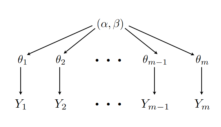
Whats nice about this is that conditional distribution of \(\theta_j \mid Y_j, a,b\sim \text{Beta}(a+y_j, \beta+n_j-y_j)\) which we saw earlier. The diagram below,Figure 3.1, provides a visual for the schematic.
Figure 3.1: From https://math.la.asu.edu/~prhahn/lect7.pdf
An important note on this model is that because the \(\theta_j\) term, known as a “random effect”, is the intermediate variable on the path from the prior parameters to the observed outcomes \(Y_j\), then all the \(Y_j\)’s are independent of one another given that we know \(\mu_1, \mu_2, \ldots, \mu_m, a, b\), which is known as conditional independence.
Choosing a hyperprior such that \(\Pr(a,b)\sim(a+b)^{-5/2}\) turns out to be convenient, as it implies a roughly
3.6.1 Another way to think about random effects
So far, we have discussed the “hierarchical model” and the random effect as being motivated from a predictive perspective. Certain groups have effects unique to that group, and we want to account for this. For example, different regions of the U.S. would have unique random effects that can increase predictive power of a model. The random effects are also often analysed to see if we can glean information about the different groups.
Part of the predictive magic of random effects in a regression can be explained via a regularization (aka “shrinkage”) perspective. This means our estimate of the means for different groups get pulled closer to one another, a nice byproduct of the estimating process of a random effect term considering the variances of other groups in the study concurrently and a good reason to pursue this type of model. Even if every observation has its own random effect (i.e. every observation has a unique variance term), the random effect is estimated considering all the other groups (individual observations in this case), so the estimates for all the random effects pulls closer to the overall mean effect as if there was a single shared term. Shrinking individual random effects to be closer to the overall average is a form of bias-variance tradeoff. We intentionally make individual random effect estimates less accurate (more biased) so that are more stable/precise.
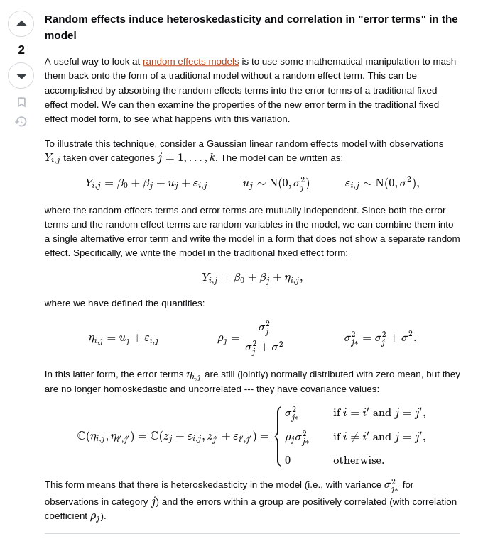
Aside from the predictive benefits of random effects that arise via shrinkage/regularization, we can also motivate random effects through a statistical model “error” analysis. Conceptually, the “random effect” term (the randomly drawn variance term added to each group) can be impactful through its effect on the error term. Unequal variances (aka heteroskedasticity) in the error term are induced because different observations now have different variance terms, depending on which group they belong too. Correlations between observations are also induced, because observations within a group will now covary together based, with the strength based on the magnitude of the random effect! for example, if the random effect is much larger than the independently (at each observation) drawn noise \(\varepsilon ~ N(0, \sigma^2)\), the observations within the groups will vary together almost perfectly. in the other direction, they will covary very little. Observations from different groups will not see their error terms change concurrently. This excellent stackoverflow answer goes into more detail on these points.
Explanation on error term view of random effects.
To use baseball as an example, consider the following scenario. Say we are predicting player value and wanna see how value differs by position. Let’s say the random effect for catchers is much higher than for second basemen (for example). this is the heteroscedacity, as noise term varies with the position. we are less certain about our predictions for catchers. because catchers and second basemen have unique random effects with different magnitudes, predictions for catchers will tend to be more similar to each other than to other positions, hence the “correlated” error within groups.
Of course, the random effects induce certain forms of correlation in the errors, which depends on the group assignment. More general analyses to account for correlated errors or heteroskedastic errors should still be pursued, as we will see in chapter 8.
What do we have to do to sample from this problem? The prior we have chosen for \(a,b\) is not a conjugate prior meaning we cannot use wikipedia. This means we will have to use some sort of MCMC techniques, with the method suggested by Richard Hahn’s notes being a Metropolis-within-Gibbs sampling technique. We sample from the marginal distribution of
So that is a lot of math which gives us the form of the numerator for the marginal distribution of the \(a,b\) hyperparameters. However, as we warned earlier, the integral in the denominator is gnarly and we do need it unfortunately. After all, we want probabilities. To do so, we follow slide 58 of Richard Hahn’s notes and implement the following Metropolis algorithm to generate samples of \(\Pr(a,b\mid y)\) sequentially:
Initialize \(a^{(1)}\) and \(b^{(1)}\). We are not raising anything to any power here, but rather making a chain of numbers.
Propose \(a'\sim \text{uniform}(a^{(s)}/2, 2a^{(s)} )\). This step updates our initial guess \(a^{(1)}\) by picking a number (with equal probability) anywhere between \(a^{(1)}/2\) and \(2a^{(1)}\) .
Evaluate our proposal according to the equations derived above. Do so by first choosing \(u\sim \text{uniform}(0,1)\) as our proposal comparison (if our proposal is less likely than a random number between 0 and 1, we feel confident throwing it away and staying where we were, vice versa if greater). So, if \(u<\frac{\Pr(a', b^{(s)}\mid y)}{\Pr(a^{(s)},b^{(s)}\mid y)}\times \frac{a^{(s)}}{a'}\) then \(a^{(s+1)}\) takes on the value of \(a'\), otherwise it remains \(a^{(s)}\).
Propose \(b'\sim \text{uniform}(b^{(s)}/2, 2b^{(s)} )\). This step updates our initial guess \(b^{(1)}\) by picking a number (with equal probability) anywhere between \(b^{(1)}/2\) and \(2b^{(1)}\) .
Evaluate our proposal according to the equations derived above. Do so by first choosing \(u\sim \text{uniform}(0,1)\) as our proposal comparison (if our proposal is less likely than a random number between 0 and 1, we feel confident throwing it away and staying where we were, vice versa if greater). So, if \(u<\frac{\Pr(a^{(s+1)}, b'\mid y)}{\Pr(a^{(s+1)},b^{(s)}\mid y)}\times \frac{b^{(s)}}{b'}\) then \(b^{(s+1)}\) takes on the value of \(b'\), otherwise it remains \(b^{(s)}\).
We had mentioned earlier this was going to be a Metroplis within Gibbs sampler, but where is the Gibbs? For those sharper than Demetri, it might be obvious given that we know the full conditional form of \(\theta_j\) and that we now have samples from the distribution of \(\Pr(a,b\mid y)\) that the Gibbs step is natural. The Gibbs step is:
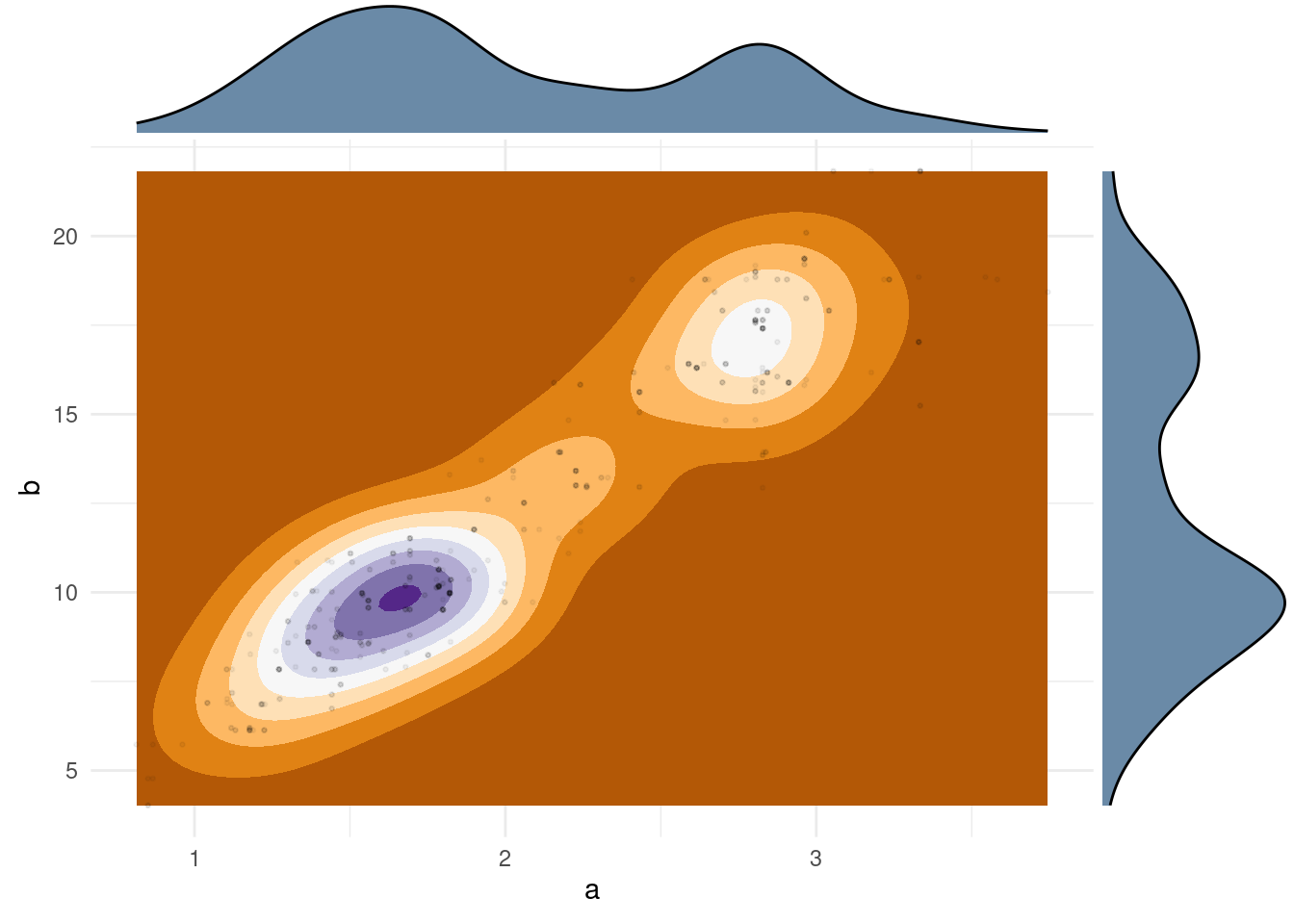
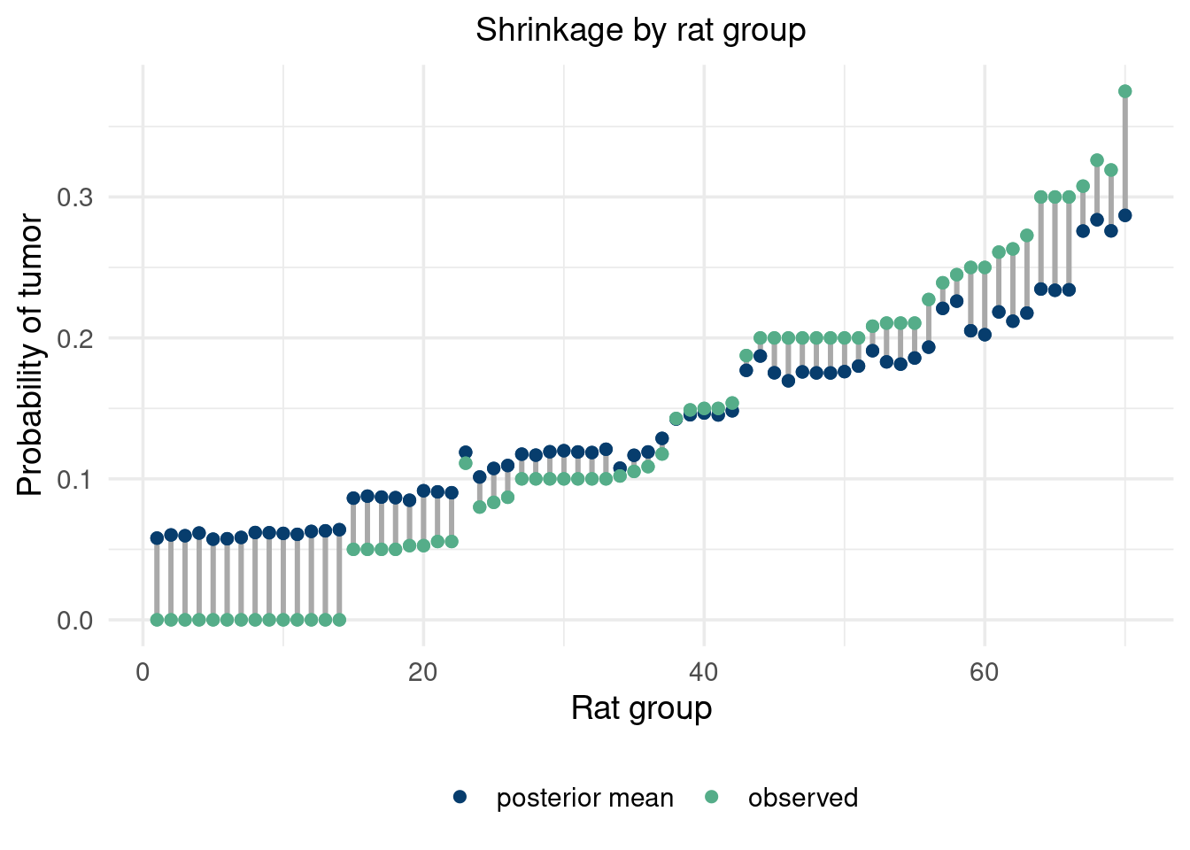
So what did it do? The above plot shows the posterior distribution of \(a\) and \(b\). Letting the sampler run for longer can show if we are not accurately sampling if there are drastic changes in that distribution. While studying the hyperparameters is an important diagnostic, we set out to study rats, so let’s get back to business. Let’s explore visually by looking at the distribution of a few different rat groups \(\theta_j\) values, which will tell us our “new belief” in their probability of developing tumors. The orange dashed line is the posterior probability, and the green solid line is the observed proportion of tumors.
Code to showcase the shrinkage properties of the model.
Note, the \(\theta_j\) are the probabilites of developing cancer for each group. To actually draw observations (i.e. the count of cancer in each group), we would sample from the posterior predictive, which in this case is conveniently \(\Pr(\tilde{y}_j^{(s)}\mid y_j)\sim \text{binomial}(n_j, \theta_j^{(s)})\)16.
16 A posterior predictive distribution is concerned with defining the distribution of future \(y\)’s (or whatever variable you are using to define the data you are modeling) given the \(y\)’s we have already observed. Essentially, the posterior predictive replaces the denominator in Bayes rule (see Equation 3.3) with the posterior distribution of \(\theta\), not the prior. I.e.
where the bottom row is the posterior predictive. Generally, we approximate the posterior predictive using our Monte Carlo draws from the posterior as plug in estimates.
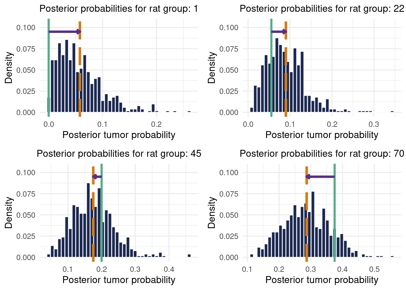
Here is another nifty way to visualize the shrinkage for every rat group.
Click here for full code
plot_shrink =data.frame(actual = y_m/n_m, quant =c(rep('observed', m), rep('posterior', m)),mean_posterior =colMeans(theta_vals[(N_MC-500):N_MC,]), iter=seq(from=1, to=m))%>%#rep(seq(from=1, to = n_sim),2))%>%mutate(diff =c(actual-mean_posterior))%>%arrange(actual)%>%ggplot(aes(x=iter, y=diff))+geom_segment( aes(x=iter, xend=iter, y=actual, yend=actual-diff), color='#A9A9A9',lwd=1)+ylab('Probability of tumor')+geom_point(aes(x=iter, y=mean_posterior, color='#073d6d'), size=2)+geom_point(aes(x=iter, y=actual, color='#55AD89'), size=2)+# uncomment for the overall means# geom_hline(aes(yintercept = mean(y_m/n_m)), color='#55AD89', lwd=1.25, lty=1)+# geom_hline(aes(yintercept = mean(theta_vals)), color='#d47c17', lwd=1.25, lty=2)+theme_minimal(base_size=14)+xlab('Rat group')+ggtitle('Shrinkage by rat group')+scale_color_manual(values=c('#073d6d', "#55AD89"), label=c('posterior mean', 'observed'), name='')+scale_shape_manual(values=c(1,2,3,4))+theme(plot.title=element_text(hjust=0.5, size=14), legend.position="bottom")plot_shrink
Another one
So we see some shrinkage to the overall mean! This is a cool example of between group and within group variability. The model provides a balance between the two types of variation and these shrinkage plots provide a nice visual.
3.6.2 Computational issues
MCMC can be slow and sometimes have a hard time converging to the truth. We will not discuss any of these methods in detail, but here are some approaches that are computationally focused. Approaches like Hamiltonian Monte Carlo are designed to work better to estimate complex posterior distributions (Neal 1996). Even more outside the box are tools that aim to bypass the likelihood + prior formulation and its focus on parameters. (Hahn, Martin, and Walker 2018) argues that the predictive distribution is what we really care about in Bayesian inference, and propose an approach for bypassing the posterior (and thus the expensive MCMC computations) and greatly speeding up the computation of the predictive distribution. Without going into detail, a key realization of the paper is that the posterior predictive can be characterized via other statistical tools rather than a Monte Carlo approximation. (Fong, Holmes, and Walker 2023) build off (Hahn, Martin, and Walker 2018), also proposing to center Bayesian posterior inference as a consideration uncertainty from the predictive distribution of future data conditioned on the \(n\) observed data \(\Pr(\mathbf{Y}_{n+1:\infty}\mid \mathbf{Y}_{1:n})\). They provide a blueprint for how to do this that we omit here. This approach allows us to bypass the likelihood and prior specifications, is potentially computationally more efficient, and is focused on prediction of future values conditioned on observables, which is arguable the greatest strength of the Bayesian paradigm.
NumPyro introduction: A newer probabilistic programming language (in Python) built off JAX that seems pretty sweet. People seem pysched about it.
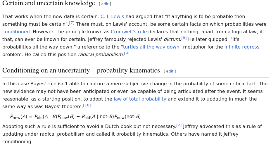
Jeffrey updating (probability kinematics) (wiki page): This is an approach to updating your posterior when your not really sure about your data. rather than the usual Bayesian updating regime of prior \(+\) data (evidence) \(\rightarrow\) posterior, aka, from Equation 3.2, \(\Pr(B) = \frac{\Pr(B\mid A)\cdot\Pr(A)}{\Pr(A\mid B)}\), where we condition on the event happening. Above we calculated the probability of no school given that we know it snowed in the morning. What if the data we condition on isn’t certain, i.e. there is some probability it is not snowing17? In this case, we can condition on potential observed data Now, (see here for a primer) we look at \(\Pr(B)_{\text{posterior}} = \sum_{i}\Pr(B\mid A_i)_{\text{prior}}\Pr(A_i)_{\text{posterior}}\) . For example, \[\Pr(B)_{\text{posterior}} = \Pr(B\mid A)\times \Pr(A)_{\text{posterior}}+\Pr(B\mid \text{not A})\times (1-\Pr(A))\], with the kicker being that \(\Pr(A)\) is now a subjective probability, set by the researcher as an attempt to quantify uncertainty in the evidence itself. For example, in the example we previously used, we (R. C. Jeffrey 1957) and (R. Jeffrey 2004) devise this approach, and (Diaconis and Zabell 1982) provides a thorough inspection of the Jeffreys conditioning approach. Interestingly, this is from Richard Jeffrey, the philosopher, not Harold Jeffreys, of Jeffreys prior fame. There is a cool connection with “Alpha-fold 1”, which netted a 2024 Nobel prize, see here(Hamelryck and Mardia 2025). This paper actually came out a few years after alpha-fold. Old ideas become new, sometimes even unknowingly. In a similar spirit, (Rappold, Lavine, and Lozier 2007) invoke subjective likelihoods. Their data did not lend itself to any realistic likelihood \(\left[\mathcal{L}(\mathbf{y}\mid\theta)\right]\) model, so they instead inferred the likelihood by consulting an expert to get a series of posteriors for \(\Pr(\theta\mid \mathbf{y}_i)\), where each \(\mathbf{y}_i\) is a different dataset. From these series of posteriors, an approximate likelihood for \(\mathbf{y}\) is derived using an algorithm developed in the paper.
Probabilities on probabilities on …
17 It may be snowing at your home, but maybe your school got nothing. You don’t really know without further inquiry. In the southwest, very localized storms (hail in one spot of town and sunny a mile away) is actually pretty normal.
Albert, Jim et al. 2009. Bayesian Computation with r. Vol. 2. Springer.
Albert, Jim, and Jingchen Hu. 2019. Probability and Bayesian Modeling. Chapman; Hall/CRC.
Blackwell, David. 1969. Basic Statistics. McGraw-Hill New York.
Carpenter, Bob, Andrew Gelman, Matthew D Hoffman, Daniel Lee, Ben Goodrich, Michael Betancourt, Marcus Brubaker, Jiqiang Guo, Peter Li, and Allen Riddell. 2017. “Stan: A Probabilistic Programming Language.”Journal of Statistical Software 76: 1–32.
Casella, George, and Roger Berger. 2002. Statistical Inference: Second Edition. CRC Press.
Diaconis, Persi, and Sandy L Zabell. 1982. “Updating Subjective Probability.”Journal of the American Statistical Association 77 (380): 822–30.
Duane, Simon, Anthony D Kennedy, Brian J Pendleton, and Duncan Roweth. 1987. “Hybrid Monte Carlo.”Physics Letters B 195 (2): 216–22.
Fong, Edwin, Chris Holmes, and Stephen G Walker. 2023. “Martingale Posterior Distributions.”Journal of the Royal Statistical Society Series B: Statistical Methodology 85 (5): 1357–91.
Gamerman, Dani, and Hedibert F Lopes. 2006. Markov Chain Monte Carlo: Stochastic Simulation for Bayesian Inference. Chapman; Hall/CRC.
Gelman, Andrew, John B Carlin, Aki Vehtari Stern Hal S, and Donald B Rubin. 2013. Bayesian Data Analysis. Chapman; Hall/CRC.
Gelman, Andrew, and Cosma Rohilla Shalizi. 2013. “Philosophy and the Practice of Bayesian Statistics.”British Journal of Mathematical and Statistical Psychology 66 (1): 8–38.
Gelman, Andrew, Daniel Simpson, and Michael Betancourt. 2017. “The Prior Can Often Only Be Understood in the Context of the Likelihood.”Entropy 19 (10): 555.
Green, Peter J. 1995. “Reversible Jump Markov Chain Monte Carlo Computation and Bayesian Model Determination.”Biometrika 82 (4): 711–32.
Gubernatis, James E. 2005. “Marshall Rosenbluth and the Metropolis Algorithm.”Physics of Plasmas 12 (5).
Hahn, P Richard, Ryan Martin, and Stephen G Walker. 2018. “On Recursive Bayesian Predictive Distributions.”Journal of the American Statistical Association 113 (523): 1085–93.
Hamelryck, Thomas, and Kanti V Mardia. 2025. “Unfolding AlphaFold’s Bayesian Roots in Probability Kinematics.”arXiv Preprint arXiv:2505.19763.
He, Jingyu, and P Richard Hahn. 2023. “Stochastic Tree Ensembles for Regularized Nonlinear Regression.”Journal of the American Statistical Association 118 (541): 551–70.
Hoff, Peter D. 2009. A First Course in Bayesian Statistical Methods. Vol. 580. Springer.
Jaynes, Edwin T. 2003. Probability Theory: The Logic of Science. Cambridge university press.
Jeffrey, Richard. 2004. Subjective Probability: The Real Thing. Cambridge University Press.
Jeffrey, Richard C. 1957. Contributions to the Theory of Inductive Probability. Princeton University.
McElreath, Richard. 2018. Statistical Rethinking: A Bayesian Course with Examples in r and Stan. Chapman; Hall/CRC.
Neal, Radford M. 1996. “Monte Carlo Implementation.” In Bayesian Learning for Neural Networks, 55–98. Springer.
Rappold, Ana Grohovac, Michael Lavine, and Susan Lozier. 2007. “Subjective Likelihood for the Assessment of Trends in the Ocean’s Mixed-Layer Depth.”Journal of the American Statistical Association 102 (479): 771–80.
Tarone, Robert E. 1982. “The Use of Historical Control Information in Testing for a Trend in Proportions.”Biometrics, 215–20.
Williams, Christopher KI, and Carl Edward Rasmussen. 2006. Gaussian Processes for Machine Learning. Vol. 2. 3. MIT press Cambridge, MA.