Gaussian Processes for Machine Learning:(Williams and Rasmussen 2006) is a cool textbook on Gaussian processes.
Bayesian Optimization:(Garnett 2023) is a good tutorial on Bayesian optimization, which includes a lot of mathematical detail as well.
Linear Models in Statistics:(Rencher and Schaalje 2008) is a good place to learn a lot of the linear algebra necessary to understand methodological statistical work.
Machine learning: a probabilistic perspective (version 1):(Murphy 2012) provide a thorough examination of many seminal topics in machine learning, with well motivated differentiation between different tools. In particular, this book casts many machine learning methods in terms of the output being a sum of many functions of the inputs and the parameters, which are learned from the data. Understanding this “adaptive basis” framework is a crucial step to a thorough comprehension of many modern statistical tools.
Modern Data Science with R:(Baumer, Kaplan, and Horton 2017) is an introduction to data analytics, and is a nice resource for data visualization. Demetri’s first statistics book. Has a big emphasis on baseball data and one of the authors was even a college player!
Python for Data Science: This bookdown project is a nice introduction to data analytics using Python.
Probability Theory: The Logic of Science:(Jaynes 2003) talks about the philosophy behind probability and Bayesian statistics.
Basic Statistics:(Blackwell 1969) is a classic statistical textbook.
All of Statistics and All of Non-Parametric Statistics: Both by the esteemed Larry Wasserman (Wasserman 2004) & (Wasserman 2006).
Introduction to Mathematical Statistics:(Hogg et al. 2013) A personal favorite undergraduate/graduate statistical text.
A Guide on Data Analysis :(Nguyen 2020) is a great bookdown with thorough explanations on a lot of topics.
Causal Inference: The Mixtape:(Cunningham 2021) have a nice bookdown as well. This is a really nice and accessible introduction to causal inference with many applications in economics and sociology.
Counterfactuals and Causal Inference:(Morgan 2015) provide a more thorough rundown of the basis of causal inference, again with applications to the social sciences.
Statistics and Causal Inference:(Holland 1986) provide a really elegant overview of the fundamental difficulties in causal analyses. Here is a link to this highly recommended (and fairly brief, by academic standards) read.
Identification for Prediction and Decision:(Manski 2009) is a good primer on statistical identification and with applications to the social sciences.
Data Analysis for Social Science: A Friendly and Practical Introduction:(Llaudet and Imai 2022) is another application book designed for quantitative social science.
Probability and Bayesian Modeling:(Albert and Hu 2019) is a nice book on Bayesian modeling with a specific focus on baseball applications. Albert and Hu wrote a few nice Bayesian textbooks with baseball applications, and there are actually a lot of baseball data you can scrape easily using the R package associated with the book.
Stats of 1:This initiative is promoting the idea that studies with only 1 person, where data on the individual constitutes the population, is the way to go for future medical research. Worth a glance at least.
Fancy data tables in R: A cool bookdown on how to make cool visuals in R.
D3.JS in observable:observable page with tutorials on how to make cool interactive visuals for webpages.
Bayesian data analysis blog: Blog from Danielle Navarro, focusing on Bayesian pharmacology. Fun writing style with cool plots and well thought out analyses.
R data science blog: Blog from Andrew Heiss with beautiful visualizations.
Another blog on Bayesian statistics and data science: This blog from Brian Lookabough has some really cool entries with fun data examples and interesting teaching points made via simulation. Additionally, the aesthetic appeal of the blog posts is high, and Brian does a good job documenting a proper data analysis workflow in the code process, which is a good trait for a young professional data science eager to enter the industry.
storytelling with data: A cool handbook on data visualization by Cole Nussbaumer Knaflic. Good suggestions we try and follow, even if she makes the graphics in Excel!
A shoutout is also due for Andrej Prsa’s “Modeling” course given at Villanova in spring 2018, which motivated some topics included in this course that we do not often see in a statistics course. Other useful courses for the authors whose content/assignments helped motivate some of the topics or were the source of different datasets include classes taught by Sebastien Motsch, Nicolas Lanchier, Shuang Zhou, and Eric Kostelich at Arizona State University, as well as courses taught by Georgia Papaefthymiou-Davis, Michael Posner, and David Chuss at Villanova University.
General statistical and modeling discussions with Drew Herren, Richard Hahn, and Rafael Alcantara have been very helpful in shaping the contents of this course (knowingly or unknowingly to them). Similar discussions with JJ Ruby and the R&D department department with the Houston Astros, as well as with former colleagues Bryce Barclay, Vincent Mutolo, and Hezekiah Grayer also warrant significant praise.
Finally, we owe a great deal of debt to the wonderful stochtree project, the hard work of Andrew Herren,Richard Hahn, Jared Murray, and others. This project is a valiant effort and will hopefully help more people have access to BART, the most talked about model in these notes that we very strongly advocate for.
# Super helpful function #https://stackoverflow.com/questions/5831794/opposite-of-in-exclude-rows-with-values-specified-in-a-vector '%!in%'<-function(x,y)!('%in%'(x,y)) RMSE <-function(m, o){ sqrt(mean((m - o)^2)) } normalize <-function(x, na.rm=T){ return((x-min(x))/(max(x)-min(x))) }
14.4 Accumulated datasets. A lot of these are weather related but not all.
A good source for looking at cool data (most of which are publicly available records) is city-data. Tidytuesday provides a lot of free and fairly clean datasets on github.
Chapter 1 data
Lake Erie ice coverage: The data are from the National Oceanic and Atmospheric Administration (noaa) government site and describe the percentage ice coverage Lake Erie achieves in a given year. Specifically, the following link will bring you directly to the .txt file on noaa’s site. Also have data for lake superior, and it’s pretty easy to download historical data for any of the great lakes.
There is data for both Arabica and Robusta beans, across many countries and professionally rated on a 0-100 scale. All sorts of scoring/ratings for things like acidity, sweetness, fragrance, balance, etc - may be useful for either separating into visualizations/categories or for modeling/recommenders.
These data are from Kuhn and Johnson (2020) and contain an abbreviated training set for modeling the number of people (in thousands) who enter the Clark and Lake L station.
The date column corresponds to the current date. The columns with station names (Austin through California) are a sample of the columns used in the original analysis (for file size reasons). These are 14 day lag variables (i.e. date - 14 days). There are columns related to weather and sports team schedules.
The station at 35th and Archer is contained in the column Archer_35th to make it a valid R column name.
chicago_train.csv
Fast food per 10,000 by state: From business insider. Describes the number of fast-food restaurants per state as of 2018.
Netflix recommender data: Data describing 100 movies with 500 ratings each (though not all by the same users). Subset of the gigantic Netflix million dollar prize data. Collected from kaggle.
netflix_movies.csv
Chapter 3 data
Rat tumor data: The data describe 71 groups of rats from (Tarone 1982) and whether or not these rats develop a tumor.
rat-tumors.csv
2020 US polling data: Data from fivethirtyeight about polling data for the 2020 U.S. election by state. Also include results from 2016 US election.
2020_fullpolls.csv
Ben Simmons 3pt shooting percentage for career: This data can be found from basketball-reference, espn, or nba.com, amongst other places. It is simply Ben Simmon’s 3PT FG percentage every year of his NBA career.
Chapter 4 data
Villanova campus coordinates Data from Jefferson Toro, and centered around the center of campus. Distance between buildings in meters.
nova.txt
Chapter 5 data
Flu data??: From Sam’s website?
Chapter 6 data
Whatever for the semi-syntetic data
Restaurant ratings: Demetri’s personal ratings for restaurants in places he’s lived or visited long enough to try a few different spots.
restaurant_ratings.csv
Chapter 7 data
Gas prices in the U.S. by state: These data were scraped from gas buddy by Jerome Goh, a graduate student at Arizona State University. Images of the time series of prices for each state were pulled from gas buddy and digitized.A visual of the gas price data is at the bottom of this page.
Wide format: gas_merged_wide.csv and long: Gasbuddy_data_ALL.csv
Squirrel census: The data are from TidyTuesday May 23, 2023 and are a collection of data on squirrel signtings in central park New York.
The Squirrel Census is a multimedia science, design, and storytelling project focusing on the Eastern gray (Sciurus carolinensis). They count squirrels and present their findings to the public. The dataset contains squirrel data for each of the 3,023 sightings, including location coordinates, age, primary and secondary fur color, elevation, activities, communications, and interactions between squirrels and with humans.
squirrel_subset.csv
Marijuana legalization data: Data on whether or not marijuana is legal in every U.S. state as of September 2022. Additional data include GDP and income per state. “personal_expend_state.csv” includes information on expenditures for each state over time.
personal_expend_state.csv and marijuana_legal.xlsx
Fast food data in the U.S.: Data describing fast food restaurants per 10,000 people across U.S. states in 2018, from business insider. Data also include income and population data by state in 2018.
fastfood.csv
Chapter 8 data
LPAA Tribolium Beetle data: Data from (Brozak et al. 2024) (from this github link) describing larvae, pupae, and adult flour beetle populations in multiple experiments.
tribolium_data_pilot.xlsx
Demetri’s walking data: From May 2021 to August 2022, Demetri’s iPhone 12 Mini recorded walking data on the daily, and we present that data here. The data are smoothed a lot to make the example more palatable, whether or not that was a smart thing to do is another story for another day.
demetri_walk.csv
Economics course grades at Michigan State University: From the Wooldridge R package and (Woolridge 2010). Data describing the grades of economic students in a Michigan State University economics course, with information recorded on every student.
econmath.csv
Effect of alcohol drinking on students GPA: Data are from (Onyper et al. 2012), which can be found at this link. The data describe college student’s GPAs, as well as information on their alcohol usage, whether or not they take early classes, their sleep levels, their stress levels, and other variables.
sleep_study_data.csv
Chapter 9 data
Demetri’s overall health data: The data are again collected on Demetri’s health data, this time collecting data on his sleep patterns, heart rate, time in bed, cycling activity, swimming activity, and a few other covariates.
demetri_sleepdata.csv
Spotify song data: The data are from TidyTuesday Jan 21, 2020. The data describe songs on spotify spanning many decades with information on the artist, track, danceability, energy, valence, key, loudness, acousticness, instrumentalness, chart ranks, and other features.
spotify_songs.csv
Chapter 10 data:
2019 NFL QB data: Data on 2019 NFL regular season quarterbacks. Data include passer rating, ESPN’s QBR statistic, accuracy, passing yards, rushing yards, and other attributes. The data are from ESPN.
qb_2019data.csv
Olive oil in Italy: The data are from (Terfloth and Gasteiger 2001) and can be found at dslabs. It describes 8 fatty acides found in 572 olive oils from different regions of Italy.
olive_oil.csv
Self reported heights: The data are also from dslabs, this time under the heights tab, including respondents reported height and sex.
Bad U.S. driver data: The data are from fivethirtyeight and have different covariates describing the driving behaviours across U.S. states from 2009-2012.
bad-drivers.csv
Chapter 11 data
Election forecast data: The data are a collection of 2020 & 2016 polling data from fivethirtyeight, 2012, 2016, and 2020 U.S. presidential election results, and U.S. demographics by state as of 2017 according to the US census.
cleaned_election_data.csv
NBA “RAPTOR” ratings: These data describe “RAPTOR” from fivethirtyeight, which is a (now defunct) basketball projection system and its associated data.
modern_RAPTOR_by_player.csv
US city data: The data are from Kaggle (and a github repo) and describe data on 343 major U.S. cities from 2022, these data are:
Population
Average Rental Price
Median Rental Price
Unemployment Rate
Per Capita Income
Air Quality
Walk, Transit, and Bike Scores
Cost of Living
Price Parity
Median Commute Time
Latitude, Longitude
us_cities.csv
TV character personality data: The data are from Tidy Tuesday August 16, 2022 and describe personality scores of characters from different TV shows. We present a subset of the data for 262 characters that include the personality traits “opinionated”, “emotional”, “bold”, “expressive”, “funny”, and “suspicious”.
tv_characters.csv is used, but TV_myers_briggs.csv and tv_show_personality.csv have more data.
Chapter 12 data
Spam or Ham data: The data are from (Lantz 2019) and can be found on Rob McCulloch’s website. The data is a list of text messages with the classification of “spam” or “ham” (with ham being a legitimate message).
sms_spam.csv
Pets data: The data are from (Brown et al. 2005), and are hosted here. They come from a survey of Californians in 2003 asking whether or not they own a dog, while also recording attributes about the respondents, such as age, gender, ethnicity, income, and other things.
pets_data.csv
UnBARTed territory: The Bartchelor data: These data describe the tv show “The Bachelor”, describing data on contestants on the show over the years, including where they place, when they get a 1 on 1 date, and their demographics at the time the show aired. The data are from here.
bach_data.csv and bachelor_full.csv
Airline traffic data: The data describe U.S. airline traffic data in 2019 and 2020. The data can be found from the bureau of transportation statistics.
travel_2020.csv
Hurricane forecast data: Data from the forecasts of Michael Mann research group at the University of Pennsylvania.
hurricane_forecast.csv
NFL ELO data: The data are from NF ELO app and describe the ELO ratings of NFL teams as of December 7, 2024. Information also includes color codes of teams and a link to their logos, which could create really cool tables or graphs.
nfelo-power-rankings-dec7-2024.csv
Walking data: Data collected in March 2025 on Demetri & his anonymous crew’s step count data. Demetri & Co. ultimately triumphed in what turned out to be a brutal back & forth contest.
boys_walk_anon.csv
Arizona weather data: The data describe different meteorological attributes in Maricopa County, Arizona, from the University of Arizona. This includes the maximum daily temperature, the mean dewpoint, the minimum temperature, and many more.
Phoenix_weather.csv
Lake Erie daily surface temperature: The data are from the “Average Surface Water Temperature (GLSEA)” page offered by noaa.gov. They describe annual average surface temperatures of Lake Erie over the years, collected daily. You can choose other Great Lakes to both visualize and download off their easy to use website.
erie_temps.csv
Conclusion chapter data
Automobile mortality data: Data in the U.S. about mortality data for drivers over/under 21 years old. The idea being when alcohol is legalized there would be a discontinuous bump in alcohol related car fatalities. The data can be found on this blog and were originally published in (Carpenter and Dobkin 2009).
df_alcohol_mort.csv
Smoking expenditure data: These data were sourced from the tidysynth R package. However, the data are from the famous synthetic control paper (Abadie, Diamond, and Hainmueller 2010) that looked at the effect of California tobacco smoking laws. Useful for a study of synthetic controls or difference in difference.
smoking.csv
Workforce attrition data: A cool dataset to study would (the fictional) workforce retention at IBM dataset, which looks at if employees terminate. If they don’t terminate, they are right censored since we do not measure how long they stay at IBM.
workforce_attrition.csv
Additional data we are looking for uses for
COVID 19 data: A collection of data per state on U.S. states regarding cases, deaths, vaccination, population, and a “stringency” index. The data were sourced from the New York Times for the deaths, cases, and population (), Bloomberg for vaccinations, and (Hallas et al. 2021) for the stringency index. This one was curated by Demetri, lwk took a while.
US_covid_data.csv
TV show personality additionals: Additional data include “notability” on 889 TV characters and Meyers-Briggs personality scores for 14,224 TV characters.
TV_myers_briggs.csv and tv_show_personality.csv
Europe beer drinking data: The data describe beer drinking in litres per capita from 1969 to 2016 across different European countries. The data are from the World Health Organization.
beer.csv
Pokemon data: The data are from this Pokemon git-repo. They include data on 801 pokemon characters including their classification, skill attributes, and matchup strengths against other characters. The RokemonR-package also hosts these data.
pokemon.csv
Wage data: These data are sourced from the ISLR R package(Gareth et al. 2013). Data was manually assembled by Steve Miller, of Inquidia Consulting (formerly Open BI). From the March 2011 Supplement to Current Population Survey data.The data are cleaned from the original source such that the features are already one-hot encoded. The data describe the wages of Mid-Atlantic male workers with attributes defining the year of data procurement, the marital status of workers, their ethnicity, degree information, and field of work. Indicators for health level and health insurance are also included.
health_insurance_outcome.csv
US news college data: From (Gareth et al. 2013), describing data on US universities used by the USnews ranking systems. Unfortunately, we do not have the US news indices to validate if we could learn their algorithm. The USnews index would also be interesting to study to see if it is truly predictive. Of maybe even more interest is to explore if the US news index (and subsequently the ranking) cause the school to achieve more prestige than its academics warrant. Link here.
colleges.csv
Soil data: The data are from the agridat R package and describe soil resitivities as a function of North and Eastern coordinates. The data are originally from “Visualizing data” (Cleveland 1993).
cleveland_soil.csv
Minnesota barley data: Again from the agridat R package. Describe yields of barley at different Minnesota farming locations over different years as a function of weather conditions that year. Originally from (Immer and Henderson 1943), put together in (Wright 2013).
Delivery data: From the modeldata R package. 10,012 orders from a restaurant and their time to delivery.
deliveries.csv
NBA shot log data: These data describe nba shot logs and are from kaggle. Download data from there as it is sorta large ~16MB. The data describe shot locations for an NBA season, including information about who the player shooting the ball is, the distance to the hoop, the result of the shot, the closest defender, the distance to the closest defender, the time in game, the time in the shotclock, the quarter of the game, and the score of the game at the time of the shot. Many applications come to mind.
If anyone is interested
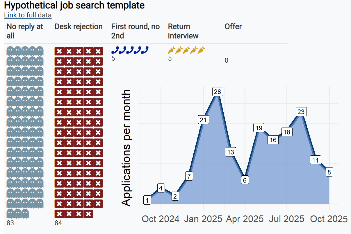
Demetri job search data:
demetri_24_jobapps.xlsx
Here is a cool visual that didn’t fit in anywhere else:
A fun idea would be to merge the plots the two previous code-snipped made on the same plot by stapling the time plot onto the emoji plot. See Figure 14.1.
Problems with calling local images from directory. Figure out…
suppressMessages(library(htmltools))suppressMessages(library(htmlwidgets))image_html <- tags$img(src ="https://demetripapakostas.com/img/hel_mist4.png",width ="90px", height ="auto", style ="display:inline-block; border:none; outline:none; position: relative; bottom: -90px; left: 40%; z-index:1; background-color:#f8f9fa;")image_html2 <- tags$img(src ="https://demetripapakostas.com/pics/time_plot_jobs2.svg",width ="515px", height ="auto",style ="display:inline-block; border:none; outline:none; position: relative; bottom: -225px; left: 17%; z-index:1; background-color:#f8f9fa;")# 2. Wrap the <img> tag within a <div> tag using htmltools::div()div_with_img <-div(image_html, style="margin: 0 auto; height:0px;width:100%;background-color:#f8f9fa")div_with_img2 <-div(image_html2, style="margin: 0 auto; height:0px;width:100%;background-color:#f8f9fa")# Convert the htmltools tag object to an HTML character stringhtml_string <-as.character(div_with_img)# 3. Prepend the image HTML to the widget# The 'html' argument accepts an htmltools tag object or a character stringfinal_widget <-prependContent(a2,div_with_img)#final_widgetfinal_widget <-prependContent(final_widget, div_with_img2)final_widget
Skeleton code to get the data in the correct format from the standard excel/csv template above:
expand for full code: not run
df %>%group_by(Date) %>%summarize(count =n())
A fun idea would be to merge Figure 1.2 with ?fig-viz_3 on the same plot by stapling the time plot onto the emoji plot. See below for a visual of that.
Merged plot
14.5 Visual of gas prices in the U.S. by state (unique to us!)